Example joint fit between GBM and Swift BAT
One of the key features of 3ML is the abil ity to fit multi-messenger data properly. A simple example of this is the joint fitting of two instruments whose data obey different likelihoods. Here, we have GBM data which obey a Poisson-Gaussian profile likelihoog ( PGSTAT in XSPEC lingo) and Swift BAT which data which are the result of a “fit” via a coded mask and hence obey a Gaussian ( \(\chi^2\) ) likelihood.
[1]:
import warnings

warnings.simplefilter("ignore")
import numpy as np

np.seterr(all="ignore")
[1]:
{'divide': 'warn', 'over': 'warn', 'under': 'ignore', 'invalid': 'warn'}
[2]:
%%capture
import matplotlib.pyplot as plt

np.random.seed(12345)
from threeML import *
from threeML.io.package_data import get_path_of_data_file
from threeML.io.logging import silence_console_log
[3]:
from jupyterthemes import jtplot

%matplotlib inline
jtplot.style(context="talk", fscale=1, ticks=True, grid=False)
set_threeML_style()
silence_warnings()
Plugin setup
We have data from the same time interval from Swift BAT and a GBM NAI and BGO detector. We have preprocessed GBM data to so that it is OGIP compliant. (Remember that we can handle the raw data with the TimeSeriesBuilder). Thus, we will use the OGIPLike plugin to read in each dataset, make energy selections and examine the raw count spectra.
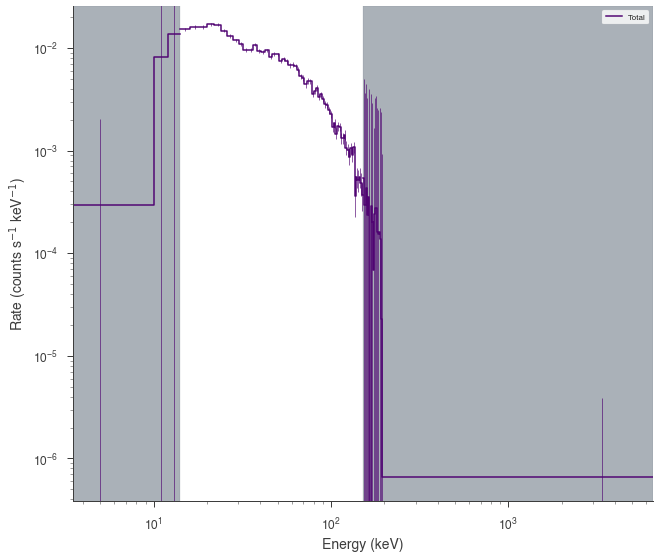
Swift BAT
[4]:
bat_pha = get_path_of_data_file("datasets/bat/gbm_bat_joint_BAT.pha")
bat_rsp = get_path_of_data_file("datasets/bat/gbm_bat_joint_BAT.rsp")

bat = OGIPLike("BAT", observation=bat_pha, response=bat_rsp)

bat.set_active_measurements("15-150")
bat.view_count_spectrum()
[4]:

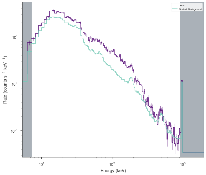
Fermi GBM
[5]:
nai6 = OGIPLike(
"n6",
get_path_of_data_file("datasets/gbm/gbm_bat_joint_NAI_06.pha"),
get_path_of_data_file("datasets/gbm/gbm_bat_joint_NAI_06.bak"),
get_path_of_data_file("datasets/gbm/gbm_bat_joint_NAI_06.rsp"),
spectrum_number=1,
)
nai6.set_active_measurements("8-900")
nai6.view_count_spectrum()
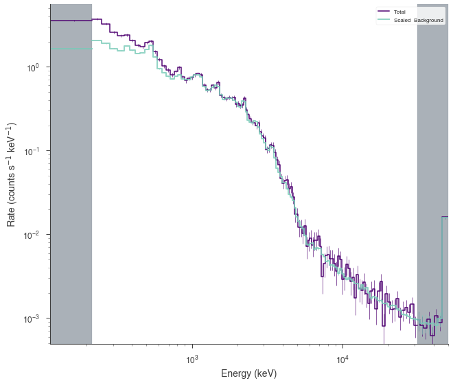
bgo0 = OGIPLike(
"b0",
get_path_of_data_file("datasets/gbm/gbm_bat_joint_BGO_00.pha"),
get_path_of_data_file("datasets/gbm/gbm_bat_joint_BGO_00.bak"),
get_path_of_data_file("datasets/gbm/gbm_bat_joint_BGO_00.rsp"),
spectrum_number=1,
)
bgo0.set_active_measurements("250-30000")
bgo0.view_count_spectrum()
[5]:

Model setup
We setup up or spectrum and likelihood model and combine the data. 3ML will automatically assign the proper likelihood to each data set. At first, we will assume a perfect calibration between the different detectors and not a apply a so-called effective area correction.
[6]:
band = Band()

model_no_eac = Model(PointSource("joint_fit_no_eac", 0, 0, spectral_shape=band))
Spectral fitting
Now we simply fit the data by building the data list, creating the joint likelihood and running the fit.
No effective area correction
[7]:
data_list = DataList(bat, nai6, bgo0)

jl_no_eac = JointLikelihood(model_no_eac, data_list)

jl_no_eac.fit()
Best fit values:
| result | unit | |
|---|---|---|
| parameter | ||
| joint_fit_no_eac.spectrum.main.Band.K | (2.75 +/- 0.06) x 10^-2 | 1 / (cm2 keV s) |
| joint_fit_no_eac.spectrum.main.Band.alpha | -1.029 +/- 0.017 | |
| joint_fit_no_eac.spectrum.main.Band.xp | (5.7 +/- 0.4) x 10^2 | keV |
| joint_fit_no_eac.spectrum.main.Band.beta | -2.41 +/- 0.18 |
Correlation matrix:
| 1.00 | 0.90 | -0.85 | 0.14 |
| 0.90 | 1.00 | -0.73 | 0.08 |
| -0.85 | -0.73 | 1.00 | -0.32 |
| 0.14 | 0.08 | -0.32 | 1.00 |
Values of -log(likelihood) at the minimum:
| -log(likelihood) | |
|---|---|
| BAT | 53.004207 |
| b0 | 553.011455 |
| n6 | 760.216969 |
| total | 1366.232632 |
Values of statistical measures:
| statistical measures | |
|---|---|
| AIC | 2740.599943 |
| BIC | 2755.306971 |
[7]:
(                                                value  negative_error  \
 joint_fit_no_eac.spectrum.main.Band.K        0.027476       -0.000557
 joint_fit_no_eac.spectrum.main.Band.alpha   -1.029036       -0.016662
 joint_fit_no_eac.spectrum.main.Band.xp     566.986887      -37.816140
 joint_fit_no_eac.spectrum.main.Band.beta    -2.410083       -0.178486

                                            positive_error      error  \
 joint_fit_no_eac.spectrum.main.Band.K            0.000581   0.000569
 joint_fit_no_eac.spectrum.main.Band.alpha        0.016928   0.016795
 joint_fit_no_eac.spectrum.main.Band.xp          34.796218  36.306179
 joint_fit_no_eac.spectrum.main.Band.beta         0.185936   0.182211

                                                       unit
 joint_fit_no_eac.spectrum.main.Band.K      1 / (cm2 keV s)
 joint_fit_no_eac.spectrum.main.Band.alpha
 joint_fit_no_eac.spectrum.main.Band.xp                 keV
 joint_fit_no_eac.spectrum.main.Band.beta                    ,
        -log(likelihood)
 BAT           53.004207
 b0           553.011455
 n6           760.216969
 total       1366.232632)
The fit has resulted in a very typical Band function fit. Let’s look in count space at how good of a fit we have obtained.
[8]:
threeML_config.plugins.ogip.fit_plot.model_cmap = "Set1"
threeML_config.plugins.ogip.fit_plot.n_colors = 3
display_spectrum_model_counts(
    jl_no_eac,
    min_rate=[0.01, 10.0, 10.0],
    data_colors=["grey", "k", "k"],
    show_background=False,
    source_only=True,
)
[8]:

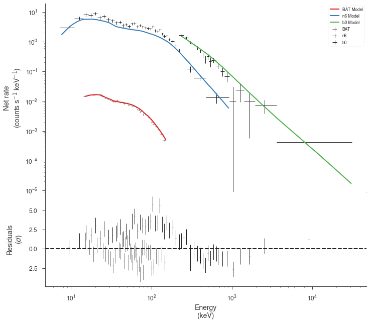
It seems that the effective areas between GBM and BAT do not agree! We can look at the goodness of fit for the various data sets.
[9]:
gof_object = GoodnessOfFit(jl_no_eac)

gof, res_frame, lh_frame = gof_object.by_mc(n_iterations=100)
[10]:
import pandas as pd

pd.Series(gof)
[10]:
total    0.00
BAT      0.00
n6       0.00
b0       0.68
dtype: float64
Both the GBM NaI detector and Swift BAT exhibit poor GOF.
With effective are correction
Now let’s add an effective area correction between the detectors to see if this fixes the problem. The effective area is a nuissance parameter that attempts to model systematic problems in a instruments calibration. It simply scales the counts of an instrument by a multiplicative factor. It cannot handle more complicated energy dependent
[11]:
# turn on the effective area correction and set it's bounds
nai6.use_effective_area_correction(0.2, 1.8)
bgo0.use_effective_area_correction(0.2, 1.8)

model_eac = Model(PointSource("joint_fit_eac", 0, 0, spectral_shape=band))

jl_eac = JointLikelihood(model_eac, data_list)

jl_eac.fit()
Best fit values:
| result | unit | |
|---|---|---|
| parameter | ||
| joint_fit_eac.spectrum.main.Band.K | (2.98 +/- 0.12) x 10^-2 | 1 / (cm2 keV s) |
| joint_fit_eac.spectrum.main.Band.alpha | (-9.84 +/- 0.26) x 10^-1 | |
| joint_fit_eac.spectrum.main.Band.xp | (3.31 +/- 0.32) x 10^2 | keV |
| joint_fit_eac.spectrum.main.Band.beta | -2.36 +/- 0.15 | |
| cons_n6 | 1.56 +/- 0.04 | |
| cons_b0 | 1.41 +/- 0.10 |
Correlation matrix:
| 1.00 | 0.95 | -0.92 | 0.31 | 0.29 | 0.62 |
| 0.95 | 1.00 | -0.82 | 0.26 | 0.26 | 0.52 |
| -0.92 | -0.82 | 1.00 | -0.36 | -0.45 | -0.77 |
| 0.31 | 0.26 | -0.36 | 1.00 | 0.04 | -0.03 |
| 0.29 | 0.26 | -0.45 | 0.04 | 1.00 | 0.47 |
| 0.62 | 0.52 | -0.77 | -0.03 | 0.47 | 1.00 |
Values of -log(likelihood) at the minimum:
| -log(likelihood) | |
|---|---|
| BAT | 40.079268 |
| b0 | 544.746813 |
| n6 | 644.532148 |
| total | 1229.358228 |
Values of statistical measures:
| statistical measures | |
|---|---|
| AIC | 2471.001202 |
| BIC | 2492.979019 |
[11]:
(                                             value  negative_error  \
 joint_fit_eac.spectrum.main.Band.K        0.029821       -0.001179
 joint_fit_eac.spectrum.main.Band.alpha   -0.983814       -0.025487
 joint_fit_eac.spectrum.main.Band.xp     330.661044      -31.342070
 joint_fit_eac.spectrum.main.Band.beta    -2.360560       -0.149352
 cons_n6                                   1.561041       -0.039060
 cons_b0                                   1.410283       -0.095224

                                         positive_error      error  \
 joint_fit_eac.spectrum.main.Band.K            0.001129   0.001154
 joint_fit_eac.spectrum.main.Band.alpha        0.024966   0.025226
 joint_fit_eac.spectrum.main.Band.xp          31.481785  31.411928
 joint_fit_eac.spectrum.main.Band.beta         0.152780   0.151066
 cons_n6                                       0.037852   0.038456
 cons_b0                                       0.095715   0.095469

                                                    unit
 joint_fit_eac.spectrum.main.Band.K      1 / (cm2 keV s)
 joint_fit_eac.spectrum.main.Band.alpha
 joint_fit_eac.spectrum.main.Band.xp                 keV
 joint_fit_eac.spectrum.main.Band.beta
 cons_n6
 cons_b0                                                  ,
        -log(likelihood)
 BAT           40.079268
 b0           544.746813
 n6           644.532148
 total       1229.358228)
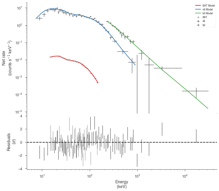
Now we have a much better fit to all data sets
[12]:
display_spectrum_model_counts(
    jl_eac, step=False, min_rate=[0.01, 10.0, 10.0], data_colors=["grey", "k", "k"]
)
[12]:

[13]:
gof_object = GoodnessOfFit(jl_eac)

# for display purposes we are keeping the output clear
# with silence_console_log(and_progress_bars=False):
gof, res_frame, lh_frame = gof_object.by_mc(n_iterations=100, continue_on_failure=True)
[14]:
import pandas as pd

pd.Series(gof)
[14]:
total    0.19
BAT      0.08
n6       0.19
b0       0.18
dtype: float64
Examining the differences
Let’s plot the fits in model space and see how different the resulting models are.
[15]:
plot_spectra(
    jl_eac.results,
    jl_no_eac.results,
    fit_cmap="Set1",
    contour_cmap="Set1",
    flux_unit="erg2/(keV s cm2)",
    equal_tailed=True,
)
[15]:
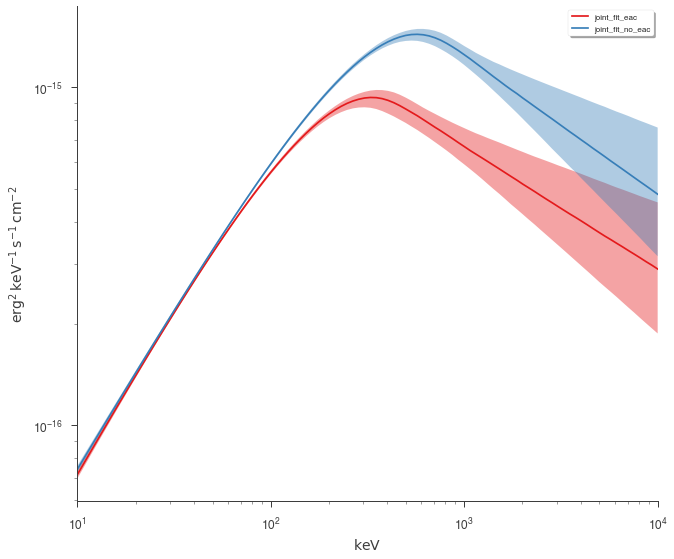

We can easily see that the models are different