Analyzing GRB 080916C

(NASA/Swift/Cruz deWilde)

To demonstrate the capabilities and features of 3ML in, we will go through a time-integrated and time-resolved analysis. This example serves as a standard way to analyze Fermi-GBM data with 3ML as well as a template for how you can design your instrument’s analysis pipeline with 3ML if you have similar data.

3ML provides utilities to reduce time series data to plugins in a correct and statistically justified way (e.g., background fitting of Poisson data is done with a Poisson likelihood). The approach is generic and can be extended. For more details, see the time series documentation.

import warnings

warnings.simplefilter("ignore")

%%capture
import matplotlib.pyplot as plt
import numpy as np

np.seterr(all="ignore")


from threeML import *
from threeML.io.package_data import get_path_of_data_file

silence_warnings()
%matplotlib inline
from jupyterthemes import jtplot

jtplot.style(context="talk", fscale=1, ticks=True, grid=False)
set_threeML_style()

Examining the catalog

As with Swift and Fermi-LAT, 3ML provides a simple interface to the on-line Fermi-GBM catalog. Let’s get the information for GRB 080916C.

gbm_catalog = FermiGBMBurstCatalog()
gbm_catalog.query_sources("GRB080916009")

Table length=1

name	ra	dec	trigger_time	t90
object	float64	float64	float64	float64
GRB080916009	119.800	-56.600	54725.0088613	62.977

To aid in quickly replicating the catalog analysis, and thanks to the tireless efforts of the Fermi-GBM team, we have added the ability to extract the analysis parameters from the catalog as well as build an astromodels model with the best fit parameters baked in. Using this information, one can quickly run through the catalog an replicate the entire analysis with a script. Let’s give it a try.

grb_info = gbm_catalog.get_detector_information()["GRB080916009"]

gbm_detectors = grb_info["detectors"]
source_interval = grb_info["source"]["fluence"]
background_interval = grb_info["background"]["full"]
best_fit_model = grb_info["best fit model"]["fluence"]
model = gbm_catalog.get_model(best_fit_model, "fluence")["GRB080916009"]

model

Model summary:

	N
Point sources	1
Extended sources	0
Particle sources	0

Free parameters (5):

	value	min_value	max_value	unit
GRB080916009.spectrum.main.SmoothlyBrokenPowerLaw.K	0.012255	0.0	None	keV-1 s-1 cm-2
GRB080916009.spectrum.main.SmoothlyBrokenPowerLaw.alpha	-1.130424	-1.5	2.0
GRB080916009.spectrum.main.SmoothlyBrokenPowerLaw.break_energy	309.2031	10.0	None	keV
GRB080916009.spectrum.main.SmoothlyBrokenPowerLaw.break_scale	0.3	0.0	10.0
GRB080916009.spectrum.main.SmoothlyBrokenPowerLaw.beta	-2.096931	-5.0	-1.6

Fixed parameters (3):
(abridged. Use complete=True to see all fixed parameters)


Linked parameters (0):

(none)

Independent variables:

(none)

Downloading the data

We provide a simple interface to download the Fermi-GBM data. Using the information from the catalog that we have extracted, we can download just the data from the detectors that were used for the catalog analysis. This will download the CSPEC, TTE and instrument response files from the on-line database.

dload = download_GBM_trigger_data("bn080916009", detectors=gbm_detectors)

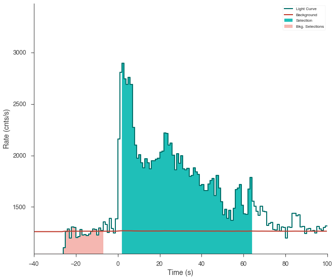
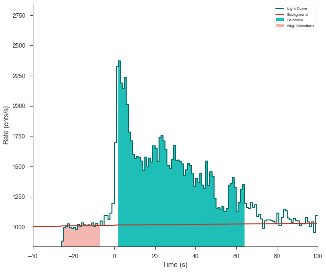
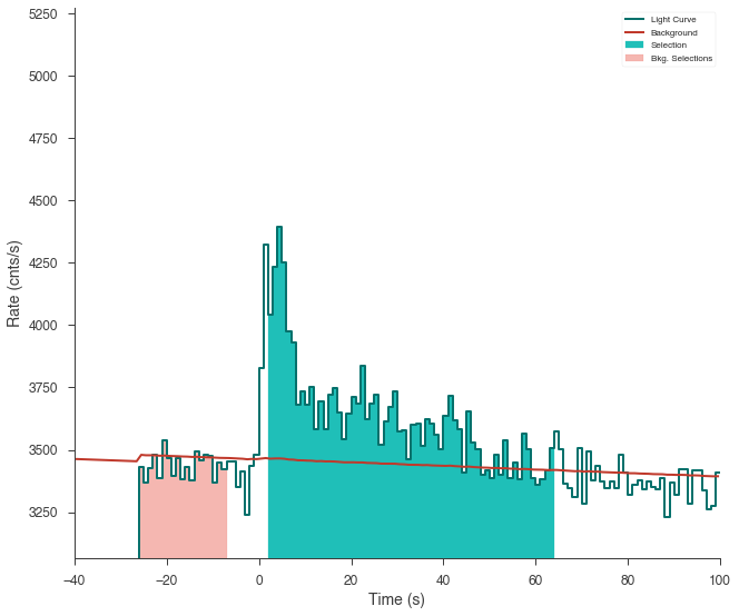
Let’s first examine the catalog fluence fit. Using the TimeSeriesBuilder, we can fit the background, set the source interval, and create a 3ML plugin for the analysis. We will loop through the detectors, set their appropriate channel selections, and ensure there are enough counts in each bin to make the PGStat profile likelihood valid.

• First we use the CSPEC data to fit the background using the background selections. We use CSPEC because it has a longer duration for fitting the background.

• The background is saved to an HDF5 file that stores the polynomial coefficients and selections which we can read in to the TTE file later.

• The light curve is plotted.

• The source selection from the catalog is set and DispersionSpectrumLike plugin is created.

• The plugin has the standard GBM channel selections for spectral analysis set.

fluence_plugins = []
time_series = {}
for det in gbm_detectors:

    ts_cspec = TimeSeriesBuilder.from_gbm_cspec_or_ctime(
        det, cspec_or_ctime_file=dload[det]["cspec"], rsp_file=dload[det]["rsp"]
    )

    ts_cspec.set_background_interval(*background_interval.split(","))
    ts_cspec.save_background(f"{det}_bkg.h5", overwrite=True)

    ts_tte = TimeSeriesBuilder.from_gbm_tte(
        det,
        tte_file=dload[det]["tte"],
        rsp_file=dload[det]["rsp"],
        restore_background=f"{det}_bkg.h5",
    )

    time_series[det] = ts_tte

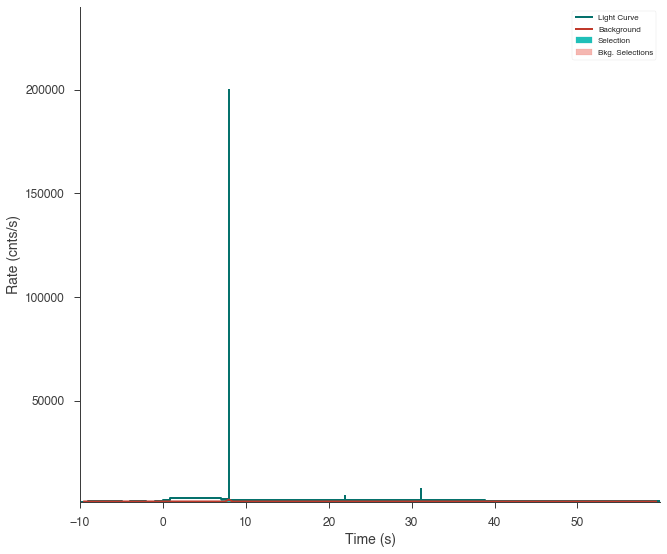
    ts_tte.set_active_time_interval(source_interval)

    ts_tte.view_lightcurve(-40, 100)

    fluence_plugin = ts_tte.to_spectrumlike()

    if det.startswith("b"):

        fluence_plugin.set_active_measurements("250-30000")

    else:

        fluence_plugin.set_active_measurements("9-900")

    fluence_plugin.rebin_on_background(1.0)

    fluence_plugins.append(fluence_plugin)

Setting up the fit

Let’s see if we can reproduce the results from the catalog.

Set priors for the model

We will fit the spectrum using Bayesian analysis, so we must set priors on the model parameters.

model.GRB080916009.spectrum.main.shape.alpha.prior = Truncated_gaussian(
    lower_bound=-1.5, upper_bound=1, mu=-1, sigma=0.5
)
model.GRB080916009.spectrum.main.shape.beta.prior = Truncated_gaussian(
    lower_bound=-5, upper_bound=-1.6, mu=-2.25, sigma=0.5
)
model.GRB080916009.spectrum.main.shape.break_energy.prior = Log_normal(mu=2, sigma=1)
model.GRB080916009.spectrum.main.shape.break_energy.bounds = (None, None)
model.GRB080916009.spectrum.main.shape.K.prior = Log_uniform_prior(
    lower_bound=1e-3, upper_bound=1e1
)
model.GRB080916009.spectrum.main.shape.break_scale.prior = Log_uniform_prior(
    lower_bound=1e-4, upper_bound=10
)

Clone the model and setup the Bayesian analysis class

Next, we clone the model we built from the catalog so that we can look at the results later and fit the cloned model. We pass this model and the DataList of the plugins to a BayesianAnalysis class and set the sampler to MultiNest.

new_model = clone_model(model)

bayes = BayesianAnalysis(new_model, DataList(*fluence_plugins))

# share spectrum gives a linear speed up when
# spectrumlike plugins have the same RSP input energies
bayes.set_sampler("multinest", share_spectrum=True)

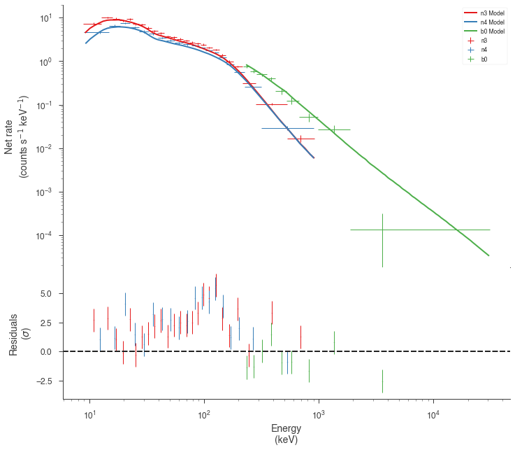
Examine at the catalog fitted model

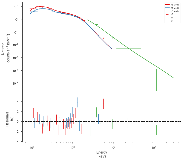
We can quickly examine how well the catalog fit matches the data. There appears to be a discrepancy between the data and the model! Let’s refit to see if we can fix it.

fig = display_spectrum_model_counts(bayes, min_rate=20, step=False)

Run the sampler

We let MultiNest condition the model on the data

bayes.sampler.setup(n_live_points=400)
bayes.sample()

  analysing data from chains/fit-.txt
Maximum a posteriori probability (MAP) point:

	result	unit
parameter
GRB080916009...K	(1.478 -0.019 +0.016) x 10^-2	1 / (cm2 keV s)
GRB080916009...alpha	-1.067 -0.016 +0.017
GRB080916009...break_energy	(2.10 +/- 0.15) x 10^2	keV
GRB080916009...break_scale	(2.3 +/- 0.4) x 10^-1
GRB080916009...beta	-2.08 -0.05 +0.04

Values of -log(posterior) at the minimum:

	-log(posterior)
b0	-1051.639405
n3	-1023.878973
n4	-1013.813454
total	-3089.331832

Values of statistical measures:

	statistical measures
AIC	6188.834118
BIC	6208.066329
DIC	6175.110102
PDIC	3.404059
log(Z)	-1348.773680

 *****************************************************
 MultiNest v3.10
 Copyright Farhan Feroz & Mike Hobson
 Release Jul 2015

 no. of live points =  400
 dimensionality =    5
 *****************************************************
 ln(ev)=  -3105.6661701539770      +/-  0.23767632803605027
 Total Likelihood Evaluations:        23321
 Sampling finished. Exiting MultiNest

Now our model seems to match much better with the data!

bayes.restore_median_fit()
fig = display_spectrum_model_counts(bayes, min_rate=20)

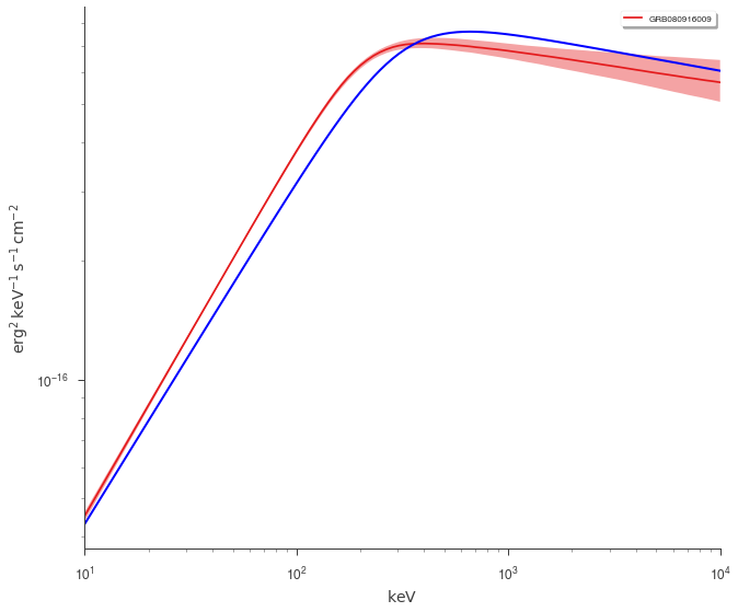
But how different are we from the catalog model? Let’s plot our fit along with the catalog model. Luckily, 3ML can handle all the units for is

conversion = u.Unit("keV2/(cm2 s keV)").to("erg2/(cm2 s keV)")
energy_grid = np.logspace(1, 4, 100) * u.keV
vFv = (energy_grid ** 2 * model.get_point_source_fluxes(0, energy_grid)).to(
    "erg2/(cm2 s keV)"
)

fig = plot_spectra(bayes.results, flux_unit="erg2/(cm2 s keV)")
ax = fig.get_axes()[0]
_ = ax.loglog(energy_grid, vFv, color="blue", label="catalog model")

Time Resolved Analysis

Now that we have examined fluence fit, we can move to performing a time-resolved analysis.

Selecting a temporal binning

We first get the brightest NaI detector and create time bins via the Bayesian blocks algorithm. We can use the fitted background to make sure that our intervals are chosen in an unbiased way.

n3 = time_series["n3"]

n3.create_time_bins(0, 60, method="bayesblocks", use_background=True, p0=0.2)

Sometimes, glitches in the GBM data cause spikes in the data that the Bayesian blocks algorithm detects as fast changes in the count rate. We will have to remove those intervals manually.

Note: In the future, 3ML will provide an automated method to remove these unwanted spikes.

fig = n3.view_lightcurve(use_binner=True)

bad_bins = []
for i, w in enumerate(n3.bins.widths):

    if w < 5e-2:
        bad_bins.append(i)


edges = [n3.bins.starts[0]]

for i, b in enumerate(n3.bins):

    if i not in bad_bins:
        edges.append(b.stop)

starts = edges[:-1]
stops = edges[1:]


n3.create_time_bins(starts, stops, method="custom")

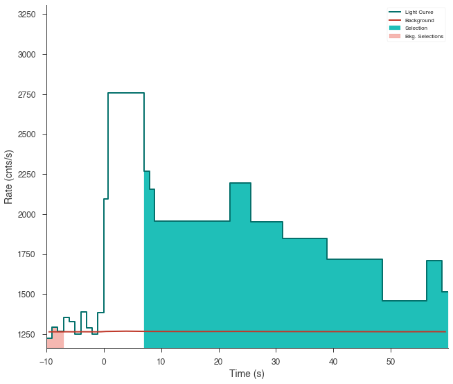
Now our light curve looks much more acceptable.

fig = n3.view_lightcurve(use_binner=True)

The time series objects can read time bins from each other, so we will map these time bins onto the other detectors’ time series and create a list of time plugins for each detector and each time bin created above.

time_resolved_plugins = {}

for k, v in time_series.items():
    v.read_bins(n3)
    time_resolved_plugins[k] = v.to_spectrumlike(from_bins=True)

Setting up the model

For the time-resolved analysis, we will fit the classic Band function to the data. We will set some principled priors.

band = Band()
band.alpha.prior = Truncated_gaussian(lower_bound=-1.5, upper_bound=1, mu=-1, sigma=0.5)
band.beta.prior = Truncated_gaussian(lower_bound=-5, upper_bound=-1.6, mu=-2, sigma=0.5)
band.xp.prior = Log_normal(mu=2, sigma=1)
band.xp.bounds = (0, None)
band.K.prior = Log_uniform_prior(lower_bound=1e-10, upper_bound=1e3)
ps = PointSource("grb", 0, 0, spectral_shape=band)
band_model = Model(ps)

Perform the fits

One way to perform Bayesian spectral fits to all the intervals is to loop through each one. There can are many ways to do this, so find an analysis pattern that works for you.

models = []
results = []
analysis = []
for interval in range(12):

    # clone the model above so that we have a separate model
    # for each fit

    this_model = clone_model(band_model)

    # for each detector set up the plugin
    # for this time interval

    this_data_list = []
    for k, v in time_resolved_plugins.items():

        pi = v[interval]

        if k.startswith("b"):
            pi.set_active_measurements("250-30000")
        else:
            pi.set_active_measurements("9-900")

        pi.rebin_on_background(1.0)

        this_data_list.append(pi)

    # create a data list

    dlist = DataList(*this_data_list)

    # set up the sampler and fit

    bayes = BayesianAnalysis(this_model, dlist)

    # get some speed with share spectrum
    bayes.set_sampler("multinest", share_spectrum=True)
    bayes.sampler.setup(n_live_points=500)
    bayes.sample()

    # at this stage we coudl also
    # save the analysis result to
    # disk but we will simply hold
    # onto them in memory

    analysis.append(bayes)

  analysing data from chains/fit-.txt
Maximum a posteriori probability (MAP) point:

	result	unit
parameter
grb.spectrum.main.Band.K	(3.8 -0.5 +0.8) x 10^-2	1 / (cm2 keV s)
grb.spectrum.main.Band.alpha	(-5.7 -1.1 +1.3) x 10^-1
grb.spectrum.main.Band.xp	(2.9 -0.5 +0.4) x 10^2	keV
grb.spectrum.main.Band.beta	-2.18 -0.13 +0.11

Values of -log(posterior) at the minimum:

	-log(posterior)
b0_interval0	-280.746107
n3_interval0	-245.079730
n4_interval0	-262.078483
total	-787.904321

Values of statistical measures:

	statistical measures
AIC	1583.921956
BIC	1599.330774
DIC	1561.202751
PDIC	1.222379
log(Z)	-344.320839

  analysing data from chains/fit-.txt
Maximum a posteriori probability (MAP) point:

	result	unit
parameter
grb.spectrum.main.Band.K	(5.663 -0.05 +0.035) x 10^-2	1 / (cm2 keV s)
grb.spectrum.main.Band.alpha	(-6.44 -0.16 +0.10) x 10^-1
grb.spectrum.main.Band.xp	(3.42 +/- 0.05) x 10^2	keV
grb.spectrum.main.Band.beta	-1.940 -0.017 +0.022

Values of -log(posterior) at the minimum:

	-log(posterior)
b0_interval1	-675.445360
n3_interval1	-643.395554
n4_interval1	-639.382744
total	-1958.223658

Values of statistical measures:

	statistical measures
AIC	3924.560631
BIC	3939.969449
DIC	3904.079074
PDIC	1.890091
log(Z)	-856.525421

  analysing data from chains/fit-.txt
Maximum a posteriori probability (MAP) point:

	result	unit
parameter
grb.spectrum.main.Band.K	(2.68 +/- 0.18) x 10^-2	1 / (cm2 keV s)
grb.spectrum.main.Band.alpha	-1.01 -0.05 +0.06
grb.spectrum.main.Band.xp	(5.4 +/- 0.9) x 10^2	keV
grb.spectrum.main.Band.beta	-2.34 -0.21 +0.22

Values of -log(posterior) at the minimum:

	-log(posterior)
b0_interval2	-317.086688
n3_interval2	-282.733765
n4_interval2	-305.860520
total	-905.680974

Values of statistical measures:

	statistical measures
AIC	1819.475262
BIC	1834.884080
DIC	1794.410451
PDIC	2.875155
log(Z)	-394.619101

  analysing data from chains/fit-.txt
Maximum a posteriori probability (MAP) point:

	result	unit
parameter
grb.spectrum.main.Band.K	(2.98 -0.4 +0.34) x 10^-2	1 / (cm2 keV s)
grb.spectrum.main.Band.alpha	(-9.5 -0.9 +0.7) x 10^-1
grb.spectrum.main.Band.xp	(3.2 -0.7 +0.6) x 10^2	keV
grb.spectrum.main.Band.beta	-1.93 -0.06 +0.09

Values of -log(posterior) at the minimum:

	-log(posterior)
b0_interval3	-292.910369
n3_interval3	-237.130733
n4_interval3	-257.028716
total	-787.069817

Values of statistical measures:

	statistical measures
AIC	1582.252949
BIC	1597.661767
DIC	1561.636052
PDIC	2.290962
log(Z)	-344.075330

  analysing data from chains/fit-.txt
Maximum a posteriori probability (MAP) point:

	result	unit
parameter
grb.spectrum.main.Band.K	(2.10 -0.10 +0.09) x 10^-2	1 / (cm2 keV s)
grb.spectrum.main.Band.alpha	(-9.62 -0.34 +0.33) x 10^-1
grb.spectrum.main.Band.xp	(3.83 -0.4 +0.34) x 10^2	keV
grb.spectrum.main.Band.beta	-2.07 +/- 0.12

Values of -log(posterior) at the minimum:

	-log(posterior)
b0_interval4	-773.580304
n3_interval4	-751.235741
n4_interval4	-741.271553
total	-2266.087599

Values of statistical measures:

	statistical measures
AIC	4540.288512
BIC	4555.697329
DIC	4520.084027
PDIC	3.289852
log(Z)	-987.193744

  analysing data from chains/fit-.txt
Maximum a posteriori probability (MAP) point:

	result	unit
parameter
grb.spectrum.main.Band.K	(3.52 -0.4 +0.20) x 10^-2	1 / (cm2 keV s)
grb.spectrum.main.Band.alpha	(-7.5 -1.0 +0.6) x 10^-1
grb.spectrum.main.Band.xp	(2.89 -0.19 +0.23) x 10^2	keV
grb.spectrum.main.Band.beta	-1.93 -0.08 +0.11

Values of -log(posterior) at the minimum:

	-log(posterior)
b0_interval5	-531.646695
n3_interval5	-521.775614
n4_interval5	-522.625707
total	-1576.048016

Values of statistical measures:

	statistical measures
AIC	3160.209347
BIC	3175.618165
DIC	3143.654827
PDIC	4.281251
log(Z)	-688.345203

  analysing data from chains/fit-.txt
Maximum a posteriori probability (MAP) point:

	result	unit
parameter
grb.spectrum.main.Band.K	(2.285 -0.028 +0.033) x 10^-2	1 / (cm2 keV s)
grb.spectrum.main.Band.alpha	(-9.735 +/- 0.021) x 10^-1
grb.spectrum.main.Band.xp	(3.07 +/- 0.06) x 10^2	keV
grb.spectrum.main.Band.beta	-2.61 -0.10 +0.09

Values of -log(posterior) at the minimum:

	-log(posterior)
b0_interval6	-606.787728
n3_interval6	-582.939490
n4_interval6	-572.662566
total	-1762.389784

Values of statistical measures:

	statistical measures
AIC	3532.892883
BIC	3548.301701
DIC	3510.679735
PDIC	0.823058
log(Z)	-770.551698

  analysing data from chains/fit-.txt
Maximum a posteriori probability (MAP) point:

	result	unit
parameter
grb.spectrum.main.Band.K	(2.01 -0.24 +0.15) x 10^-2	1 / (cm2 keV s)
grb.spectrum.main.Band.alpha	(-9.3 -1.4 +0.7) x 10^-1
grb.spectrum.main.Band.xp	(2.95 -0.4 +0.19) x 10^2	keV
grb.spectrum.main.Band.beta	-1.94 +/- 0.05

Values of -log(posterior) at the minimum:

	-log(posterior)
b0_interval7	-660.759100
n3_interval7	-637.875755
n4_interval7	-643.886733
total	-1942.521588

Values of statistical measures:

	statistical measures
AIC	3893.156491
BIC	3908.565309
DIC	3879.859181
PDIC	5.416102
log(Z)	-848.066517

  analysing data from chains/fit-.txt
Maximum a posteriori probability (MAP) point:

	result	unit
parameter
grb.spectrum.main.Band.K	(2.02 -0.08 +0.12) x 10^-2	1 / (cm2 keV s)
grb.spectrum.main.Band.alpha	(-6.6 +/- 0.6) x 10^-1
grb.spectrum.main.Band.xp	(2.55 -0.16 +0.14) x 10^2	keV
grb.spectrum.main.Band.beta	-2.08 +/- 0.06

Values of -log(posterior) at the minimum:

	-log(posterior)
b0_interval8	-697.038606
n3_interval8	-694.439788
n4_interval8	-660.999214
total	-2052.477608

Values of statistical measures:

	statistical measures
AIC	4113.068531
BIC	4128.477349
DIC	4097.894198
PDIC	2.578329
log(Z)	-895.791060

  analysing data from chains/fit-.txt
Maximum a posteriori probability (MAP) point:

	result	unit
parameter
grb.spectrum.main.Band.K	(1.6 -0.8 +0.6) x 10^-2	1 / (cm2 keV s)
grb.spectrum.main.Band.alpha	(-7.9 -2.6 +2.5) x 10^-1
grb.spectrum.main.Band.xp	(1.2 +/- 0.4) x 10^2	keV
grb.spectrum.main.Band.beta	-2.05 -0.25 +0.26

Values of -log(posterior) at the minimum:

	-log(posterior)
b0_interval9	-647.064763
n3_interval9	-615.046435
n4_interval9	-613.699612
total	-1875.810809

Values of statistical measures:

	statistical measures
AIC	3759.734933
BIC	3775.143750
DIC	3705.284947
PDIC	-40.413977
log(Z)	-817.000780

  analysing data from chains/fit-.txt
Maximum a posteriori probability (MAP) point:

	result	unit
parameter
grb.spectrum.main.Band.K	(2.03 -0.35 +0.32) x 10^-2	1 / (cm2 keV s)
grb.spectrum.main.Band.alpha	(-7.4 -1.2 +1.1) x 10^-1
grb.spectrum.main.Band.xp	(2.3 +/- 0.4) x 10^2	keV
grb.spectrum.main.Band.beta	-2.30 +/- 0.28

Values of -log(posterior) at the minimum:

	-log(posterior)
b0_interval10	-457.098760
n3_interval10	-433.945604
n4_interval10	-429.236603
total	-1320.280968

Values of statistical measures:

	statistical measures
AIC	2648.675249
BIC	2664.084067
DIC	2630.784816
PDIC	2.238113
log(Z)	-575.302011

  analysing data from chains/fit-.txt
Maximum a posteriori probability (MAP) point:

	result	unit
parameter
grb.spectrum.main.Band.K	(3.2 -1.3 +1.2) x 10^-2	1 / (cm2 keV s)
grb.spectrum.main.Band.alpha	(-4.7 -2.6 +2.4) x 10^-1
grb.spectrum.main.Band.xp	(1.32 -0.30 +0.28) x 10^2	keV
grb.spectrum.main.Band.beta	-2.32 -0.34 +0.4

Values of -log(posterior) at the minimum:

	-log(posterior)
b0_interval11	-289.545062
n3_interval11	-268.987041
n4_interval11	-252.424633
total	-810.956736

Values of statistical measures:

	statistical measures
AIC	1630.026787
BIC	1645.435605
DIC	1612.445198
PDIC	-0.055738
log(Z)	-353.431772

 *****************************************************
 MultiNest v3.10
 Copyright Farhan Feroz & Mike Hobson
 Release Jul 2015

 no. of live points =  500
 dimensionality =    4
 *****************************************************
 ln(ev)=  -792.82803152812608      +/-  0.18739380253309873
 Total Likelihood Evaluations:        17922
 Sampling finished. Exiting MultiNest
 *****************************************************
 MultiNest v3.10
 Copyright Farhan Feroz & Mike Hobson
 Release Jul 2015

 no. of live points =  500
 dimensionality =    4
 *****************************************************
 ln(ev)=  -1972.2226652101631      +/-  0.22878901983144731
 Total Likelihood Evaluations:        23065
 Sampling finished. Exiting MultiNest
 *****************************************************
 MultiNest v3.10
 Copyright Farhan Feroz & Mike Hobson
 Release Jul 2015

 no. of live points =  500
 dimensionality =    4
 *****************************************************
 ln(ev)=  -908.64405830872431      +/-  0.19283490366218359
 Total Likelihood Evaluations:        21439
 Sampling finished. Exiting MultiNest
 *****************************************************
 MultiNest v3.10
 Copyright Farhan Feroz & Mike Hobson
 Release Jul 2015

 no. of live points =  500
 dimensionality =    4
 *****************************************************
 ln(ev)=  -792.26272683488628      +/-  0.18470881232667236
 Total Likelihood Evaluations:        16799
 Sampling finished. Exiting MultiNest
 *****************************************************
 MultiNest v3.10
 Copyright Farhan Feroz & Mike Hobson
 Release Jul 2015

 no. of live points =  500
 dimensionality =    4
 *****************************************************
 ln(ev)=  -2273.0975981832712      +/-  0.19728338907242407
 Total Likelihood Evaluations:        21665
 Sampling finished. Exiting MultiNest
 *****************************************************
 MultiNest v3.10
 Copyright Farhan Feroz & Mike Hobson
 Release Jul 2015

 no. of live points =  500
 dimensionality =    4
 *****************************************************
 ln(ev)=  -1584.9734041063878      +/-  0.19845063525310230
 Total Likelihood Evaluations:        19290
 Sampling finished. Exiting MultiNest
 *****************************************************
 MultiNest v3.10
 Copyright Farhan Feroz & Mike Hobson
 Release Jul 2015

 no. of live points =  500
 dimensionality =    4
 *****************************************************
 ln(ev)=  -1774.2608522161704      +/-  0.21924060589409819
 Total Likelihood Evaluations:        28869
 Sampling finished. Exiting MultiNest
 *****************************************************
 MultiNest v3.10
 Copyright Farhan Feroz & Mike Hobson
 Release Jul 2015

 no. of live points =  500
 dimensionality =    4
 *****************************************************
 ln(ev)=  -1952.7453195973394      +/-  0.19828337035545832
 Total Likelihood Evaluations:        20957
 Sampling finished. Exiting MultiNest
 *****************************************************
 MultiNest v3.10
 Copyright Farhan Feroz & Mike Hobson
 Release Jul 2015

 no. of live points =  500
 dimensionality =    4
 *****************************************************
 ln(ev)=  -2062.6351404295297      +/-  0.19478411349480623
 Total Likelihood Evaluations:        18587
 Sampling finished. Exiting MultiNest
 *****************************************************
 MultiNest v3.10
 Copyright Farhan Feroz & Mike Hobson
 Release Jul 2015

 no. of live points =  500
 dimensionality =    4
 *****************************************************
 ln(ev)=  -1881.2138170182341      +/-  0.14646153851714061
 Total Likelihood Evaluations:        13178
 Sampling finished. Exiting MultiNest
 *****************************************************
 MultiNest v3.10
 Copyright Farhan Feroz & Mike Hobson
 Release Jul 2015

 no. of live points =  500
 dimensionality =    4
 *****************************************************
 ln(ev)=  -1324.6818345610895      +/-  0.16911819606590028
 Total Likelihood Evaluations:        14828
 Sampling finished. Exiting MultiNest
 *****************************************************
 MultiNest v3.10
 Copyright Farhan Feroz & Mike Hobson
 Release Jul 2015

 no. of live points =  500
 dimensionality =    4
 *****************************************************
 ln(ev)=  -813.80672880256611      +/-  0.14678498265643469
 Total Likelihood Evaluations:        12480
 Sampling finished. Exiting MultiNest

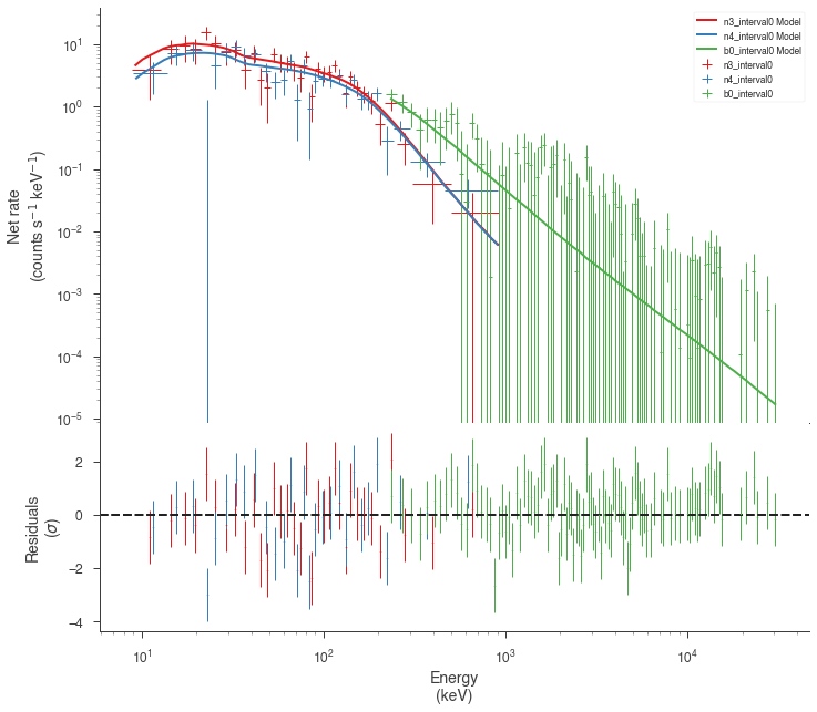
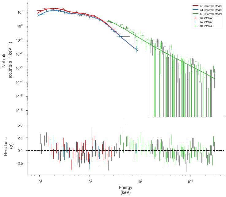
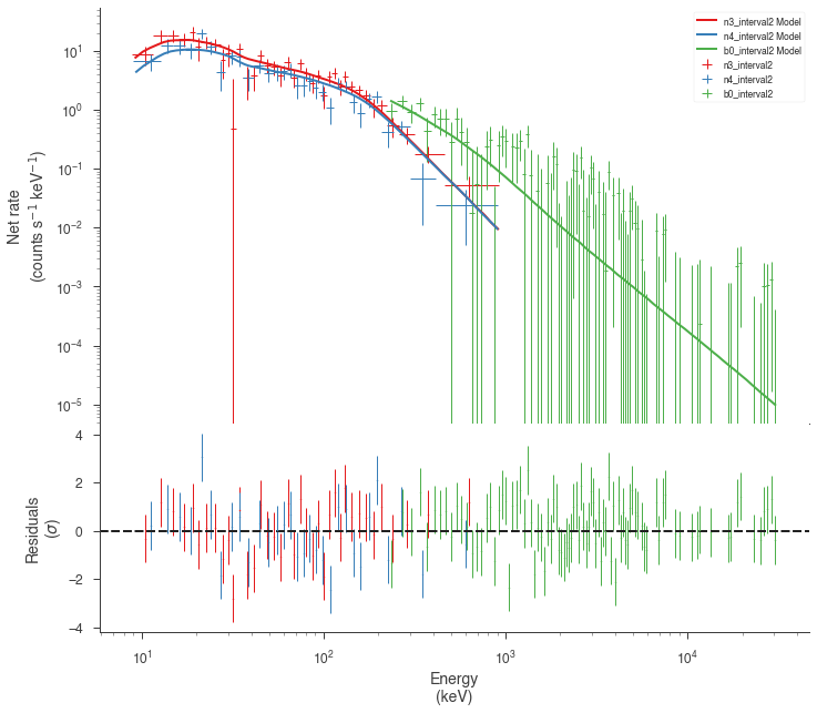
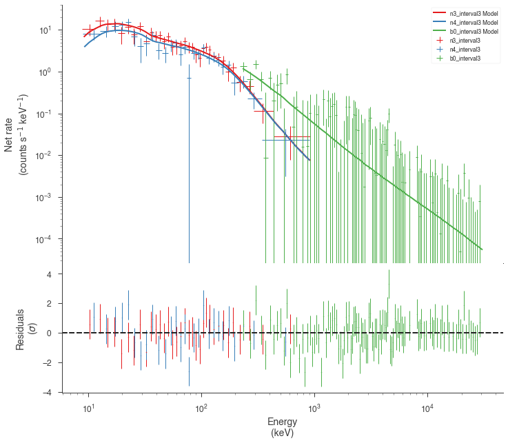
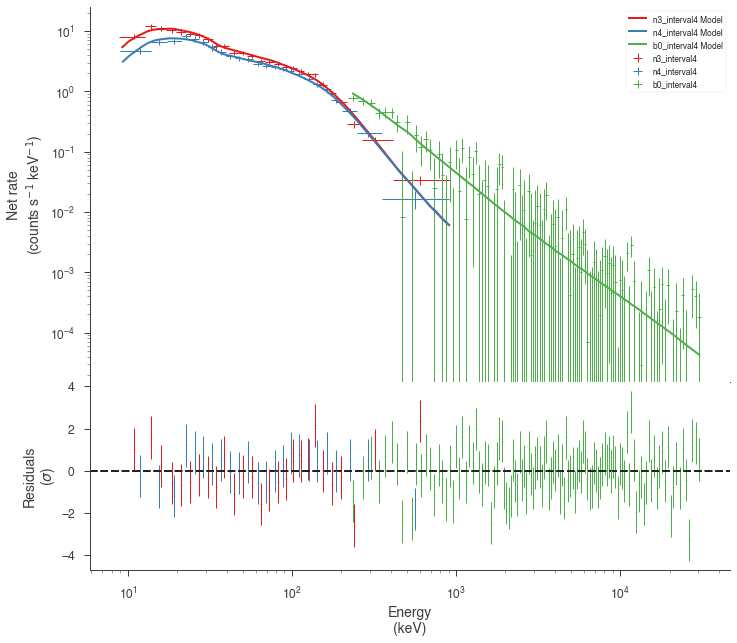
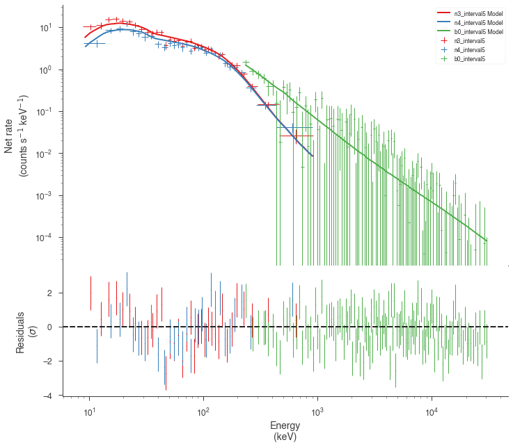
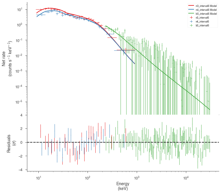
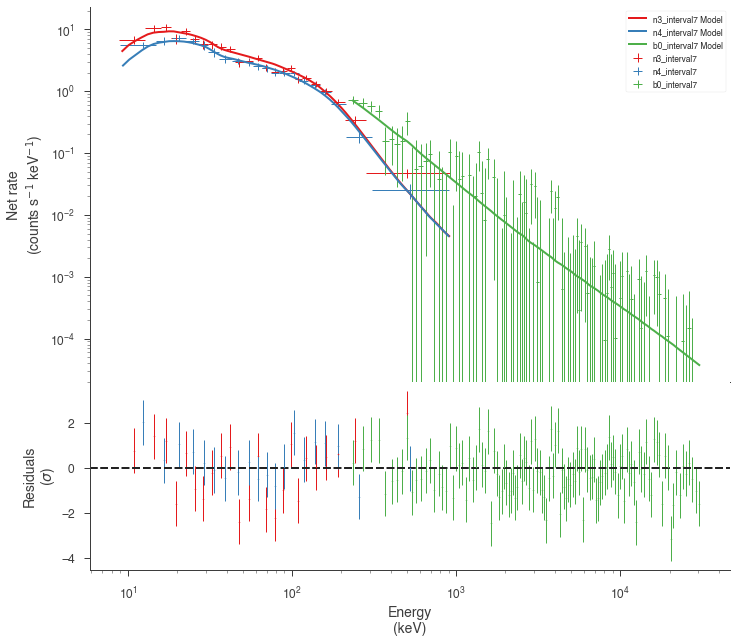
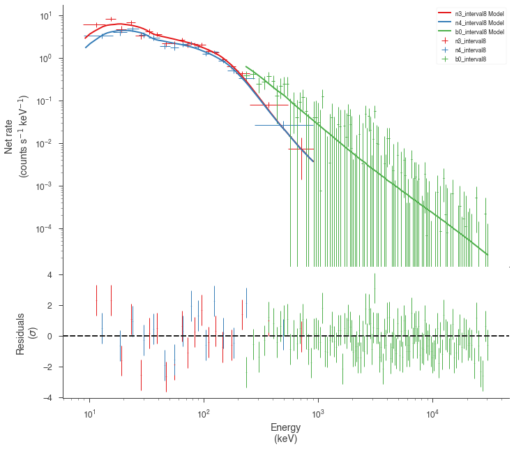
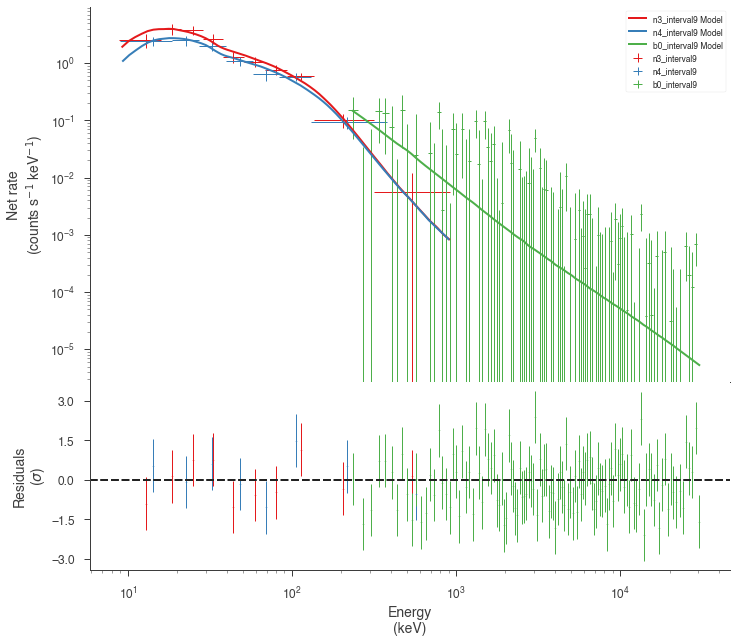
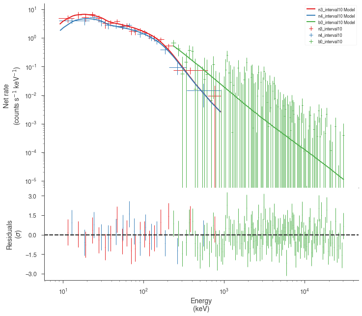
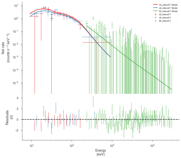
Examine the fits

Now we can look at the fits in count space to make sure they are ok.

for a in analysis:
    a.restore_median_fit()
    _ = display_spectrum_model_counts(a, min_rate=[20, 20, -99], step=False)

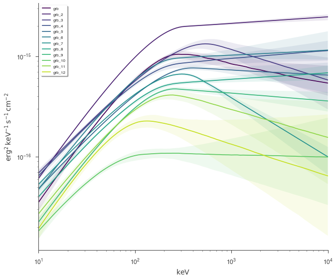
Finally, we can plot the models together to see how the spectra evolve with time.

fig = plot_spectra(
    *[a.results for a in analysis[::1]],
    flux_unit="erg2/(cm2 s keV)",
    fit_cmap="viridis",
    contour_cmap="viridis",
    contour_style_kwargs=dict(alpha=0.1),
)

This example can serve as a template for performing analysis on GBM data. However, as 3ML provides an abstract interface and modular building blocks, similar analysis pipelines can be built for any time series data.