Bayesian Sampler Examples

Examples of running each sampler avaiable in 3ML.

Before, that, let’s discuss setting up configuration default sampler with default parameters. We can set in our configuration a default algorithm and default setup parameters for the samplers. This can ease fitting when we are doing exploratory data analysis.

With any of the samplers, you can pass keywords to access their setups. Read each pacakges documentation for more details.

[1]:

from threeML import *
from threeML.plugins.XYLike import XYLike

from packaging.version import Version
import numpy as np
import dynesty
from jupyterthemes import jtplot

%matplotlib inline
jtplot.style(context="talk", fscale=1, ticks=True, grid=False)
silence_warnings()
set_threeML_style()

23:24:59 WARNING   The naima package is not available. Models that depend on it will not be         functions.py:43
                  available

         WARNING   The GSL library or the pygsl wrapper cannot be loaded. Models that depend on it  functions.py:65
                  will not be available.

         WARNING   The ebltable package is not available. Models that depend on it will not be     absorption.py:33
                  available

[2]:

threeML_config.bayesian.default_sampler

[2]:

<Sampler.emcee: 'emcee'>

[3]:

threeML_config.bayesian.emcee_setup

[3]:

{'n_burnin': None, 'n_iterations': 500, 'n_walkers': 50, 'seed': 5123}

If you simply run bayes_analysis.sample() the default sampler and its default parameters will be used.

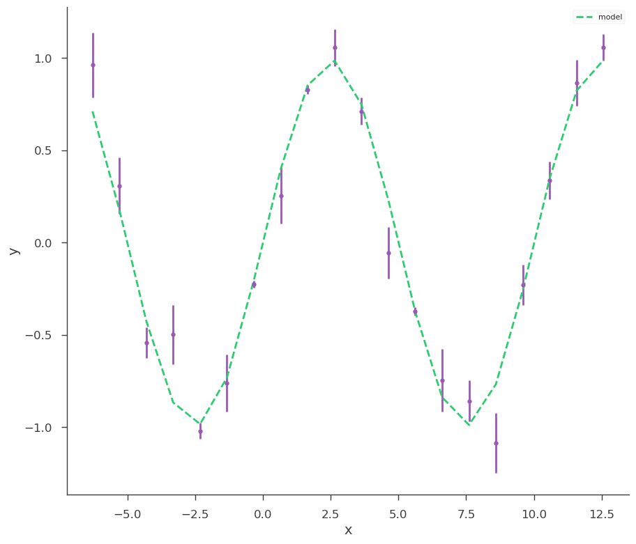
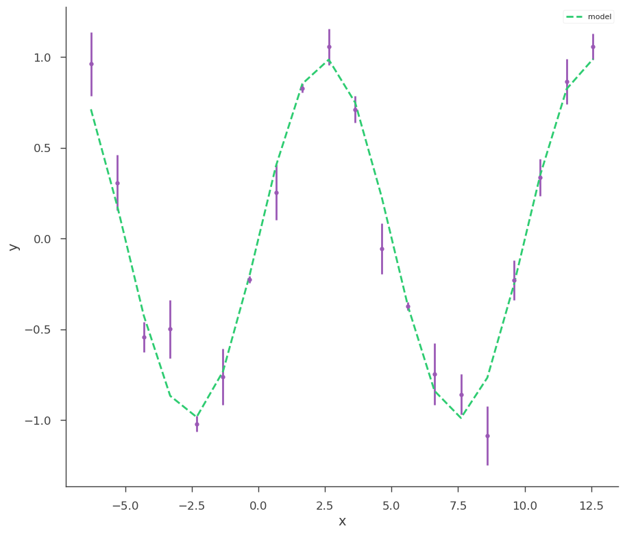
Let’s make some data to fit.

[4]:

sin = Sin(K=1, f=0.1)
sin.phi.fix = True
sin.K.prior = Log_uniform_prior(lower_bound=0.5, upper_bound=1.5)
sin.f.prior = Uniform_prior(lower_bound=0, upper_bound=0.5)

model = Model(PointSource("demo", 0, 0, spectral_shape=sin))

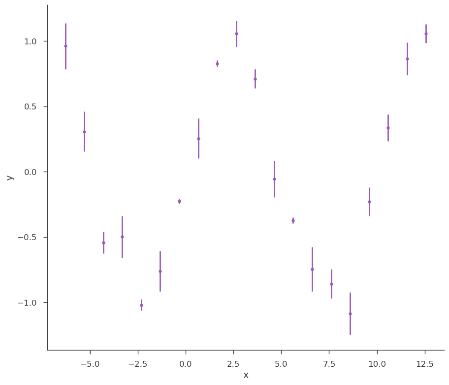
x = np.linspace(-2 * np.pi, 4 * np.pi, 20)
yerr = np.random.uniform(0.01, 0.2, 20)


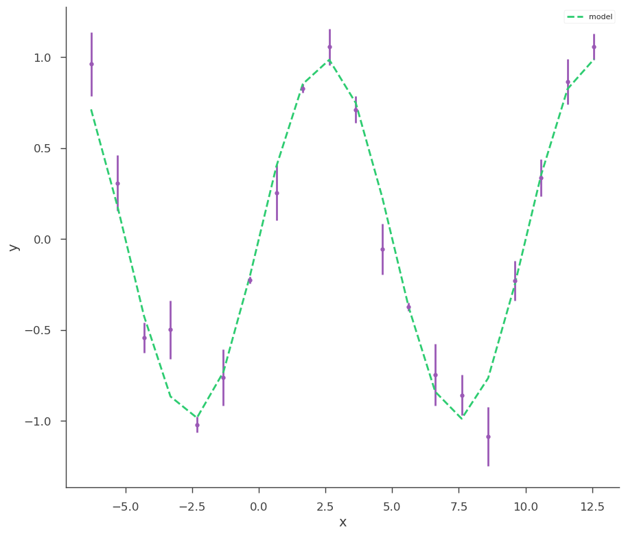
xyl = XYLike.from_function("demo", sin, x, yerr)
xyl.plot()

bayes_analysis = BayesianAnalysis(model, DataList(xyl))

23:25:01 INFO      Using Gaussian statistic (equivalent to chi^2) with the provided errors.            XYLike.py:90

23:25:02 INFO      Using Gaussian statistic (equivalent to chi^2) with the provided errors.            XYLike.py:90

../_images/notebooks_sampler_docs_5_2.png

emcee

[5]:

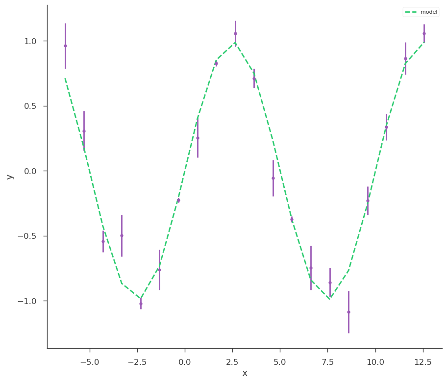
bayes_analysis.set_sampler("emcee")
bayes_analysis.sampler.setup(n_walkers=20, n_iterations=500)
bayes_analysis.sample()

xyl.plot()
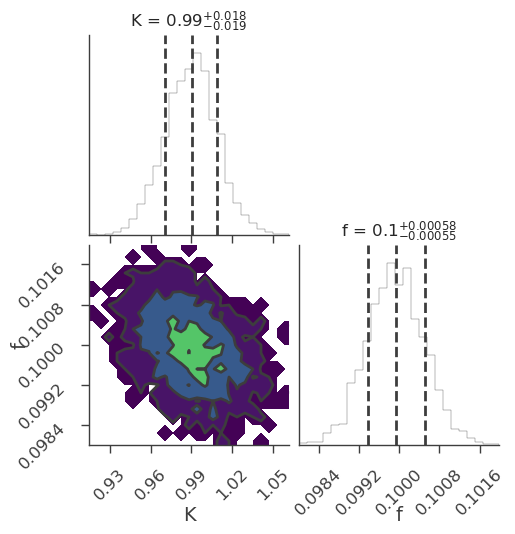
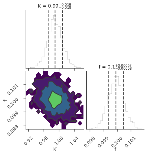
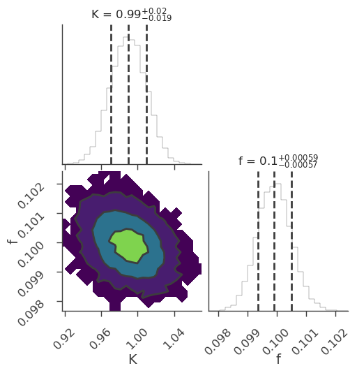
bayes_analysis.results.corner_plot()

         INFO      sampler set to emcee                                                    bayesian_analysis.py:186

23:25:04 INFO      Mean acceptance fraction: 0.7243                                            emcee_sampler.py:145

         INFO      fit restored to maximum of posterior                                         sampler_base.py:168

         INFO      fit restored to maximum of posterior                                         sampler_base.py:168

Maximum a posteriori probability (MAP) point:

	result	unit
parameter
demo.spectrum.main.Sin.K	(9.90 -0.19 +0.18) x 10^-1	1 / (keV s cm2)
demo.spectrum.main.Sin.f	(9.99 +/- 0.06) x 10^-2	rad / keV

Values of -log(posterior) at the minimum:

	-log(posterior)
demo	-12.829902
total	-12.829902

Values of statistical measures:

	statistical measures
AIC	30.365686
BIC	31.651268
DIC	29.692235
PDIC	2.014778

[5]:

../_images/notebooks_sampler_docs_7_12.png

../_images/notebooks_sampler_docs_7_13.png

../_images/notebooks_sampler_docs_7_14.png

multinest

[6]:

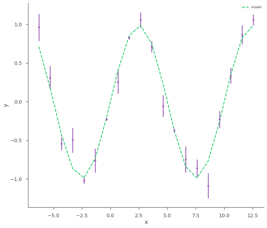
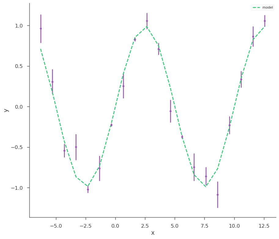
bayes_analysis.set_sampler("multinest")
bayes_analysis.sampler.setup(n_live_points=400, resume=False, auto_clean=True)
bayes_analysis.sample()

xyl.plot()
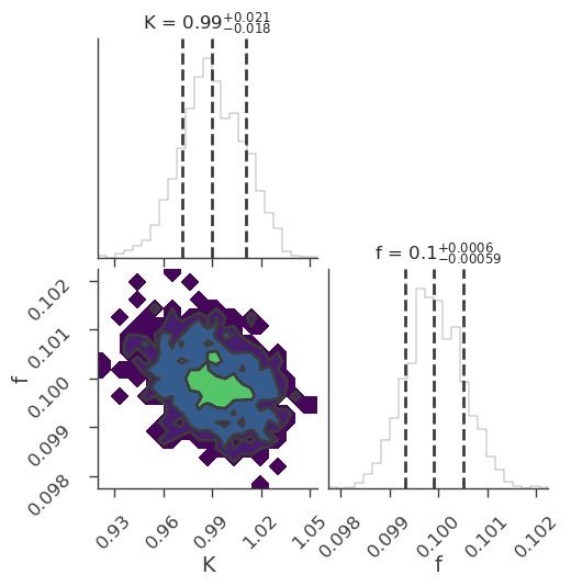
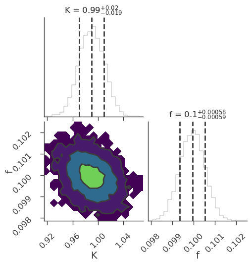
bayes_analysis.results.corner_plot()

         INFO      sampler set to multinest                                                bayesian_analysis.py:186

 *****************************************************
 MultiNest v3.10
 Copyright Farhan Feroz & Mike Hobson
 Release Jul 2015

 no. of live points =  400
 dimensionality =    2
 *****************************************************
  analysing data from chains/fit-.txt ln(ev)=  -21.613739366536066      +/-  0.13911666236546869
 Total Likelihood Evaluations:         6151
 Sampling finished. Exiting MultiNest

23:25:05 INFO      fit restored to maximum of posterior                                         sampler_base.py:168

         INFO      fit restored to maximum of posterior                                         sampler_base.py:168

Maximum a posteriori probability (MAP) point:

	result	unit
parameter
demo.spectrum.main.Sin.K	(9.90 -0.18 +0.21) x 10^-1	1 / (keV s cm2)
demo.spectrum.main.Sin.f	(9.99 +/- 0.06) x 10^-2	rad / keV

Values of -log(posterior) at the minimum:

	-log(posterior)
demo	-12.830849
total	-12.830849

Values of statistical measures:

	statistical measures
AIC	30.367581
BIC	31.653164
DIC	29.732820
PDIC	2.036253
log(Z)	-9.386728

         INFO      deleting the chain directory chains                                     multinest_sampler.py:234

[6]:

../_images/notebooks_sampler_docs_9_11.png

../_images/notebooks_sampler_docs_9_12.png

../_images/notebooks_sampler_docs_9_13.png

dynesty

[7]:

bayes_analysis.set_sampler("dynesty_nested")
bayes_analysis.sampler.setup(nlive=400)
bayes_analysis.sample()

xyl.plot()
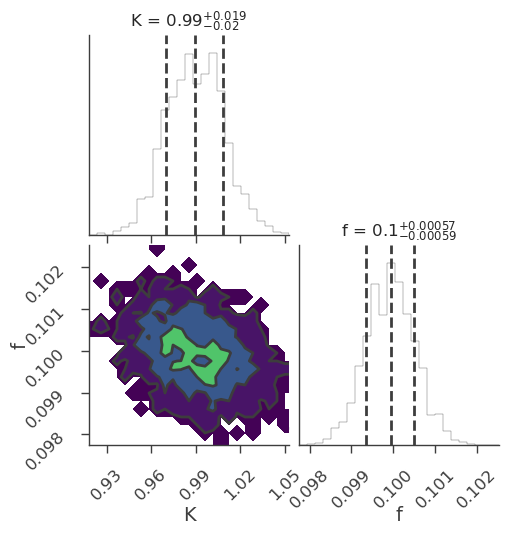
bayes_analysis.results.corner_plot()

         INFO      sampler set to dynesty_nested                                           bayesian_analysis.py:186

4003it [00:03, 1160.55it/s, +400 | bound: 11 | nc: 1 | ncall: 18297 | eff(%): 24.602 | loglstar:   -inf < -12.842 <    inf | logz: -21.806 +/-  0.141 | dlogz:  0.001 >  0.409]

23:25:09 INFO      fit restored to maximum of posterior                                         sampler_base.py:168

         INFO      fit restored to maximum of posterior                                         sampler_base.py:168

Maximum a posteriori probability (MAP) point:

	result	unit
parameter
demo.spectrum.main.Sin.K	(9.90 -0.20 +0.19) x 10^-1	1 / (keV s cm2)
demo.spectrum.main.Sin.f	(10.00 +/- 0.06) x 10^-2	rad / keV

Values of -log(posterior) at the minimum:

	-log(posterior)
demo	-12.831762
total	-12.831762

Values of statistical measures:

	statistical measures
AIC	30.369405
BIC	31.654988
DIC	29.602491
PDIC	1.971123
log(Z)	-9.470292

[7]:

../_images/notebooks_sampler_docs_11_10.png

../_images/notebooks_sampler_docs_11_11.png

../_images/notebooks_sampler_docs_11_12.png

[8]:

bayes_analysis.set_sampler("dynesty_dynamic")
bayes_analysis.sampler.setup()

if Version(dynesty.__version__) >= Version("3.0.0"):
    bayes_analysis.sample(n_effective=None)
else:
    bayes_analysis.sample(
        stop_function=dynesty.utils.old_stopping_function, n_effective=None
    )

xyl.plot()
bayes_analysis.results.corner_plot()

         INFO      sampler set to dynesty_dynamic                                          bayesian_analysis.py:186

16267it [00:13, 1208.05it/s, batch: 8 | bound: 5 | nc: 1 | ncall: 37771 | eff(%): 43.025 | loglstar: -17.747 < -12.841 < -13.106 | logz: -21.979 +/-  0.074 | stop:  0.895]

23:25:23 INFO      fit restored to maximum of posterior                                         sampler_base.py:168

         INFO      fit restored to maximum of posterior                                         sampler_base.py:168

Maximum a posteriori probability (MAP) point:

	result	unit
parameter
demo.spectrum.main.Sin.K	(9.90 -0.20 +0.19) x 10^-1	1 / (keV s cm2)
demo.spectrum.main.Sin.f	(9.99 +/- 0.06) x 10^-2	rad / keV

Values of -log(posterior) at the minimum:

	-log(posterior)
demo	-12.829911
total	-12.829911

Values of statistical measures:

	statistical measures
AIC	30.365704
BIC	31.651286
DIC	29.682828
PDIC	2.011453
log(Z)	-9.549421

[8]:

../_images/notebooks_sampler_docs_12_10.png

../_images/notebooks_sampler_docs_12_11.png

../_images/notebooks_sampler_docs_12_12.png

zeus

[9]:

bayes_analysis.set_sampler("zeus")
bayes_analysis.sampler.setup(n_walkers=20, n_iterations=500)
bayes_analysis.sample()

xyl.plot()
bayes_analysis.results.corner_plot()

         INFO      sampler set to zeus                                                     bayesian_analysis.py:186

The run method has been deprecated and it will be removed. Please use the new run_mcmc method.
Initialising ensemble of 20 walkers...
Sampling progress : 100%|██████████| 625/625 [00:03<00:00, 174.76it/s]

23:25:27 INFO      fit restored to maximum of posterior                                         sampler_base.py:168

         INFO      fit restored to maximum of posterior                                         sampler_base.py:168

Summary
-------
Number of Generations: 625
Number of Parameters: 2
Number of Walkers: 20
Number of Tuning Generations: 21
Scale Factor: 1.140697
Mean Integrated Autocorrelation Time: 3.22
Effective Sample Size: 3884.51
Number of Log Probability Evaluations: 65302
Effective Samples per Log Probability Evaluation: 0.059485

None

Maximum a posteriori probability (MAP) point:

	result	unit
parameter
demo.spectrum.main.Sin.K	(9.90 -0.20 +0.19) x 10^-1	1 / (keV s cm2)
demo.spectrum.main.Sin.f	(9.99 +/- 0.06) x 10^-2	rad / keV

Values of -log(posterior) at the minimum:

	-log(posterior)
demo	-12.829862
total	-12.829862

Values of statistical measures:

	statistical measures
AIC	30.365606
BIC	31.651188
DIC	29.711920
PDIC	2.025540

[9]:

../_images/notebooks_sampler_docs_14_12.png

../_images/notebooks_sampler_docs_14_13.png

../_images/notebooks_sampler_docs_14_14.png

ultranest

[10]:

bayes_analysis.set_sampler("ultranest")
bayes_analysis.sampler.setup(
    min_num_live_points=400, frac_remain=0.5, use_mlfriends=False
)
bayes_analysis.sample()

xyl.plot()
bayes_analysis.results.corner_plot()

23:25:28 INFO      sampler set to ultranest                                                bayesian_analysis.py:186

[ultranest] Sampling 400 live points from prior ...

[ultranest] Explored until L=-1e+01
[ultranest] Likelihood function evaluations: 6033
[ultranest]   logZ = -21.78 +- 0.08704
[ultranest] Effective samples strategy satisfied (ESS = 962.2, need >400)
[ultranest] Posterior uncertainty strategy is satisfied (KL: 0.46+-0.06 nat, need <0.50 nat)
[ultranest] Evidency uncertainty strategy is satisfied (dlogz=0.41, need <0.5)
[ultranest]   logZ error budget: single: 0.14 bs:0.09 tail:0.41 total:0.41 required:<0.50
[ultranest] done iterating.

23:25:31 INFO      fit restored to maximum of posterior                                         sampler_base.py:168

         INFO      fit restored to maximum of posterior                                         sampler_base.py:168

Maximum a posteriori probability (MAP) point:

	result	unit
parameter
demo.spectrum.main.Sin.K	(9.91 -0.20 +0.18) x 10^-1	1 / (keV s cm2)
demo.spectrum.main.Sin.f	(9.99 -0.05 +0.06) x 10^-2	rad / keV

Values of -log(posterior) at the minimum:

	-log(posterior)
demo	-12.830051
total	-12.830051

Values of statistical measures:

	statistical measures
AIC	30.365984
BIC	31.651566
DIC	29.396977
PDIC	1.868290
log(Z)	-9.460694

[10]:

../_images/notebooks_sampler_docs_16_12.png

../_images/notebooks_sampler_docs_16_13.png

../_images/notebooks_sampler_docs_16_14.png