Random Variates
When we perform a fit or load and analysis result, the parmeters of our model become distributions in the AnalysisResults object. These are actaully instantiactions of the RandomVaraiates class.
While we have covered most of the functionality of RandomVariates in the AnalysisResults section, we want to highlight a few of the details here.
[1]:
import warnings

warnings.simplefilter("ignore")
import numpy as np

np.seterr(all="ignore")
[1]:
{'divide': 'warn', 'over': 'warn', 'under': 'ignore', 'invalid': 'warn'}
[2]:
%%capture
import matplotlib.pyplot as plt
from threeML import *
[3]:
from jupyterthemes import jtplot

%matplotlib inline
jtplot.style(context="talk", fscale=1, ticks=True, grid=False)
set_threeML_style()
silence_warnings()
Let’s load back our fit of the line + gaussian from the AnalysisResults section.
[4]:
ar = load_analysis_results("test_mle.fits")
When we display our fit, we can see the parameter paths of the model. What if we want specific information on a parameter(s)?
[5]:
ar.display()
Best fit values:
| result | unit | |
|---|---|---|
| parameter | ||
| fake.spectrum.main.composite.a_1 | 2.01 +/- 0.11 | 1 / (cm2 keV s) |
| fake.spectrum.main.composite.b_1 | (-3 +/- 4) x 10^-3 | 1 / (cm2 keV2 s) |
| fake.spectrum.main.composite.F_2 | (3.2 +/- 0.4) x 10 | 1 / (cm2 s) |
| fake.spectrum.main.composite.mu_2 | (2.501 +/- 0.012) x 10 | keV |
| fake.spectrum.main.composite.sigma_2 | 1.10 +/- 0.09 | keV |
Correlation matrix:
| 1.00 | -0.85 | -0.05 | 0.03 | -0.09 |
| -0.85 | 1.00 | -0.00 | -0.02 | 0.00 |
| -0.05 | -0.00 | 1.00 | 0.00 | -0.20 |
| 0.03 | -0.02 | 0.00 | 1.00 | -0.06 |
| -0.09 | 0.00 | -0.20 | -0.06 | 1.00 |
Values of -log(likelihood) at the minimum:
| -log(likelihood) | |
|---|---|
| sim_data | 22.09818 |
| total | 22.09818 |
Values of statistical measures:
| statistical measures | |
|---|---|
| AIC | 55.559996 |
| BIC | 63.756475 |
Let’s take a look at the normalization of the gaussian. To access the parameter, we take the parameter path, and we want to get the variates:
[6]:
norm = ar.get_variates("fake.spectrum.main.composite.F_2")
Now, norm is a RandomVariate.
[7]:
type(norm)
[7]:
threeML.random_variates.RandomVariates
This is essentially a wrapper around numpy NDArray with a few added properties. It is an array of samples. In the MLE case, they are samples from the covariance matrix (this is not at all a marginal distribution, but the parameter “knows” about the entire fit, i.e., it is not a profile) and in the Bayesian case, these are samples from the posterior (this is a marginal).
The output representation for an RV are its 68% equal-tail and HPD uncertainties.
[8]:
norm
[8]:
equal-tail: (3.2 +/- 0.4) x 10, hpd: (3.2 +/- 0.4) x 10
We can access these directly, and to any desired confidence level.
[9]:
norm.equal_tail_interval(cl=0.95)
[9]:
(24.0251651631074, 39.43374603502662)
[10]:
norm.highest_posterior_density_interval(cl=0.5)
[10]:
(28.863644864483334, 34.227822547326014)
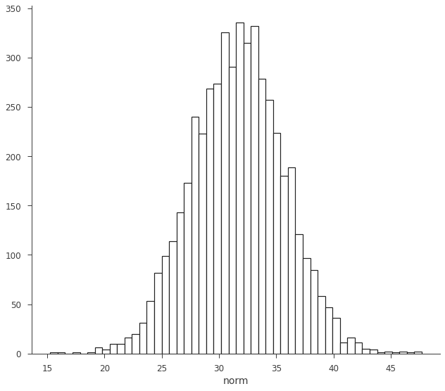
As stated above, the RV is made from samples. We can histogram them to show this explicitly.
[11]:
fig, ax = plt.subplots()

ax.hist(norm.samples, bins=50, ec="k", fc="w", lw=1.2)
ax.set_xlabel("norm")
[11]:
Text(0.5, 0, 'norm')
findfont: Font family ['sans-serif'] not found. Falling back to DejaVu Sans.
findfont: Generic family 'sans-serif' not found because none of the following families were found: Helvetica
findfont: Font family ['sans-serif'] not found. Falling back to DejaVu Sans.
findfont: Generic family 'sans-serif' not found because none of the following families were found: Helvetica
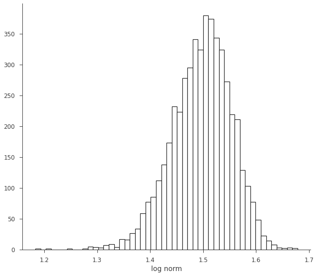
We can easily transform the RV through propagation.
[12]:
log_norm = np.log10(norm)
log_norm
[12]:
equal-tail: 1.50 -0.06 +0.05, hpd: 1.50 -0.06 +0.05
[13]:
fig, ax = plt.subplots()

ax.hist(log_norm.samples, bins=50, ec="k", fc="w", lw=1.2)
ax.set_xlabel("log norm")
[13]:
Text(0.5, 0, 'log norm')