[1]:
import warnings

warnings.simplefilter("ignore")
[2]:
%%capture
import matplotlib.pyplot as plt
import numpy as np

np.seterr(all="ignore")

from threeML import *
from threeML.io.package_data import get_path_of_data_file
[3]:
from jupyterthemes import jtplot

%matplotlib inline
jtplot.style(context="talk", fscale=1, ticks=True, grid=False)

silence_warnings()

set_threeML_style()
Constructing plugins from TimeSeries
Many times we encounter event lists or sets of spectral histograms from which we would like to derive a single or set of plugins. For this purpose, we provide the TimeSeriesBuilder which provides a unified interface to time series data. Here we will demonstrate how to construct plugins from different data types.
These utilities are helpers that allow you to reduce data to pluigns for spectral and temporal fitting. They are not plugins themselves.
Constructing time series objects from different data types
The TimeSeriesBuilder currently supports reading of the following data type: * A generic PHAII data file * GBM TTE/CSPEC/CTIME files * LAT LLE files * POLAR spectra and polarization light curves * KONUS GRB data
Note: If you would like to build a time series from your own custom data, consider creating a TimeSeriesBuilder.from_your_data() class method.
GBM Data
Building plugins from GBM is achieved in the following fashion
[4]:
cspec_file = get_path_of_data_file("datasets/glg_cspec_n3_bn080916009_v01.pha")
tte_file = get_path_of_data_file("datasets/glg_tte_n3_bn080916009_v01.fit.gz")
gbm_rsp = get_path_of_data_file("datasets/glg_cspec_n3_bn080916009_v00.rsp2")


gbm_cspec = TimeSeriesBuilder.from_gbm_cspec_or_ctime(
    "nai3_cspec", cspec_or_ctime_file=cspec_file, rsp_file=gbm_rsp
)

gbm_tte = TimeSeriesBuilder.from_gbm_tte(
    "nai3_tte", tte_file=tte_file, rsp_file=gbm_rsp
)
LAT LLE data
LAT LLE data is constructed in a similar fashion
[5]:
lle_file = get_path_of_data_file("datasets/gll_lle_bn080916009_v10.fit")
ft2_file = get_path_of_data_file("datasets/gll_pt_bn080916009_v10.fit")
lle_rsp = get_path_of_data_file("datasets/gll_cspec_bn080916009_v10.rsp")

lat_lle = TimeSeriesBuilder.from_lat_lle(
    "lat_lle", lle_file=lle_file, ft2_file=ft2_file, rsp_file=lle_rsp
)
Viewing Lightcurves and selecting source intervals
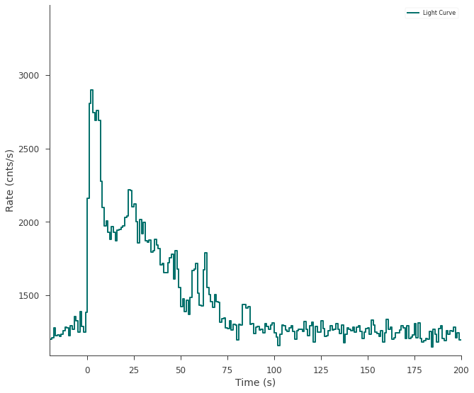
All time series objects share the same commands to get you to a plugin. Let’s have a look at the GBM TTE lightcurve.
[6]:
fig = gbm_tte.view_lightcurve(start=-20, stop=200)
findfont: Font family ['sans-serif'] not found. Falling back to DejaVu Sans.
findfont: Generic family 'sans-serif' not found because none of the following families were found: Helvetica
findfont: Font family ['sans-serif'] not found. Falling back to DejaVu Sans.
findfont: Generic family 'sans-serif' not found because none of the following families were found: Helvetica
findfont: Font family ['sans-serif'] not found. Falling back to DejaVu Sans.
findfont: Generic family 'sans-serif' not found because none of the following families were found: Helvetica
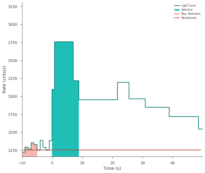
Perhaps we want to fit the time interval from 0-10 seconds. We make a selection like this:
[7]:
gbm_tte.set_active_time_interval("0-10")
fig = gbm_tte.view_lightcurve(start=-20, stop=200)
12:34:33 INFO Interval set to 0.0-10.0 for nai3_tte time_series_builder.py:291
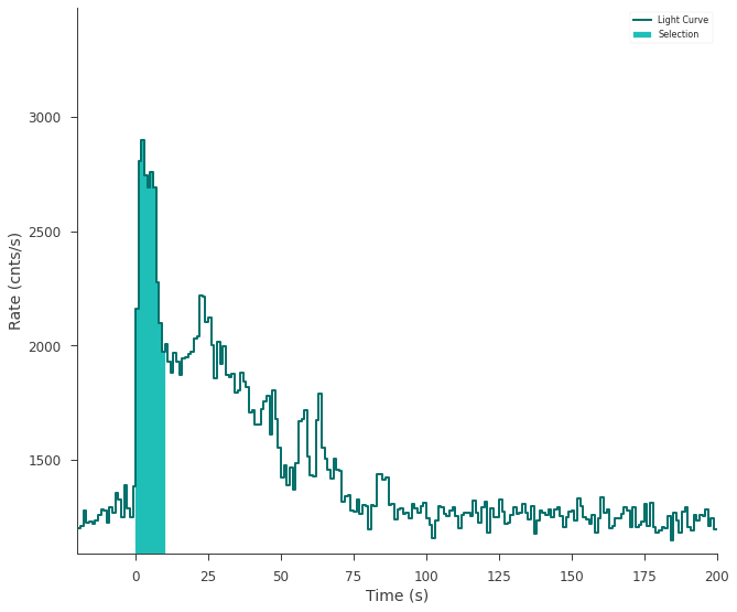
For event list style data like time tagged events, the selection is exact. However, pre-binned data in the form of e.g. PHAII files will have the selection automatically adjusted to the underlying temporal bins.
Several discontinuous time selections can be made.
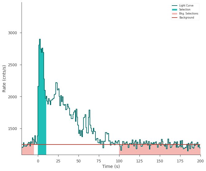
Fitting a polynomial background
In order to get to a plugin, we need to model and create an estimated background in each channel (\(B_i\)) for our interval of interest. The process that we have implemented is to fit temporal off-source regions to polynomials (\(P(t;\vec{\theta})\)) in time. First, a polynomial is fit to the total count rate. From this fit we determine the best polynomial order via a likelihood ratio test, unless the user supplies a polynomial order in the constructor or directly via the polynomial_order attribute. Then, this order of polynomial is fit to every channel in the data.
From the polynomial fit, the polynomial is integrated in time over the active source interval to estimate the count rate in each channel. The estimated background and background errors then stored for each channel.
[8]:
gbm_tte.set_background_interval("-24--5", "100-200")
fig = gbm_tte.view_lightcurve(start=-20, stop=200)
12:34:35 INFO Auto-determined polynomial order: 0 event_list.py:539
12:34:44 INFO None 0-order polynomial fit with the mle method time_series.py:459
What occurs during a fit?
In the background, the data type of the time series is analyzed (is it Poisson of Gaussian distributed?) and the time series are converted to plugins of counts / measurements vs. time. These plugins are then fit with either MLE or Bayesian methods just any other 3ML analysis. While this happens behinds the scene, it is possible to interface to these low-level operations are create your own custom background routines!
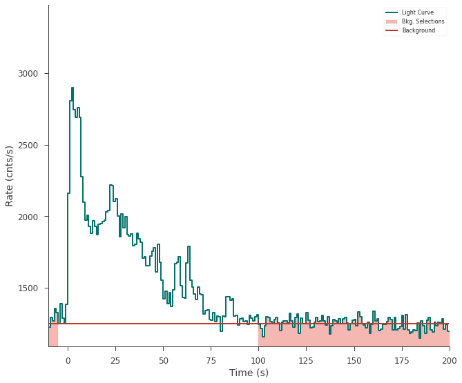
For event list data, binned or unbinned background fits are possible. For pre-binned data, only a binned fit is possible.
[9]:
gbm_tte.set_background_interval("-24--5", "100-200", unbinned=False)
12:34:45 INFO Auto-determined polynomial order: 0 event_list.py:539
12:34:53 INFO None 0-order polynomial fit with the mle method time_series.py:459
Saving the background fit
The background polynomial coefficients can be saved to disk for faster manipulation of time series data.
[10]:
gbm_tte.save_background("background_store", overwrite=True)
INFO Saved fitted background to background_store.h5 time_series.py:1064
INFO Saved background to background_store time_series_builder.py:471
[11]:
gbm_tte_reloaded = TimeSeriesBuilder.from_gbm_tte(
    "nai3_tte",
    tte_file=tte_file,
    rsp_file=gbm_rsp,
    restore_background="background_store.h5",
)
12:34:54 INFO Successfully restored fit from background_store.h5 time_series_builder.py:171
[12]:
fig = gbm_tte_reloaded.view_lightcurve(-10, 200)
Creating a plugin
With our background selections made, we can now create a plugin instance. In the case of GBM data, this results in a DispersionSpectrumLike plugin. Please refer to the Plugins documentation for more details.
[13]:
gbm_plugin = gbm_tte.to_spectrumlike()
INFO Auto-probed noise models: SpectrumLike.py:491
INFO - observation: poisson SpectrumLike.py:492
INFO - background: gaussian SpectrumLike.py:493
[14]:
gbm_plugin.display()
| 0 | |
|---|---|
| n. channels | 128 |
| total rate | 2508.771647 |
| total bkg. rate | 1253.55087 |
| total bkg. rate error | 3.250957 |
| bkg. exposure | 9.94112 |
| bkg. is poisson | False |
| exposure | 9.94112 |
| is poisson | True |
| background | profiled |
| significance | 93.530927 |
| src/bkg area ratio | 1.0 |
| src/bkg exposure ratio | 1.0 |
| src/bkg scale factor | 1.0 |
| response | None |
Time-resolved binning and plugin creation
It is possible to temporally bin time series. There are up to four methods provided depending on the type of time series being used:
Constant cadence (all time series)
Custom (all time series)
Significance (all time series)
Bayesian Blocks (event lists)
Constant Cadence
Constant cadence bins are defined by a start and a stop time along with a time delta.
[15]:
gbm_tte.create_time_bins(start=0, stop=10, method="constant", dt=2.0)
INFO Created 5 bins via constant time_series_builder.py:708
[16]:
gbm_tte.bins.display()
| Start | Stop | Duration | Midpoint | |
|---|---|---|---|---|
| 0 | 0.000412 | 2.000412 | 2.0 | 1.000412 |
| 1 | 2.000412 | 4.000412 | 2.0 | 3.000412 |
| 2 | 4.000412 | 6.000412 | 2.0 | 5.000412 |
| 3 | 6.000412 | 8.000412 | 2.0 | 7.000412 |
| 4 | 8.000412 | 10.000412 | 2.0 | 9.000412 |
Custom
Custom time bins can be created by providing a contiguous list of start and stop times.
[17]:
time_edges = np.array([0.5, 0.63, 20.0, 21.0])

starts = time_edges[:-1]

stops = time_edges[1:]

gbm_tte.create_time_bins(start=starts, stop=stops, method="custom")
INFO Created 3 bins via custom time_series_builder.py:708
[18]:
gbm_tte.bins.display()
| Start | Stop | Duration | Midpoint | |
|---|---|---|---|---|
| 0 | 0.50 | 0.63 | 0.13 | 0.565 |
| 1 | 0.63 | 20.00 | 19.37 | 10.315 |
| 2 | 20.00 | 21.00 | 1.00 | 20.500 |
Significance
Time bins can be created by specifying a significance of signal to background if a background fit has been performed.
[19]:
gbm_tte.create_time_bins(start=0.0, stop=50.0, method="significance", sigma=25)
12:35:28 INFO Created 33 bins via significance time_series_builder.py:708
[20]:
gbm_tte.bins.display()
| Start | Stop | Duration | Midpoint | |
|---|---|---|---|---|
| 0 | 0.000412 | 1.102108 | 1.101696 | 0.551260 |
| 1 | 1.102108 | 1.526892 | 0.424784 | 1.314500 |
| 2 | 1.526892 | 1.975848 | 0.448956 | 1.751370 |
| 3 | 1.975848 | 2.433242 | 0.457394 | 2.204545 |
| 4 | 2.433242 | 2.775556 | 0.342314 | 2.604399 |
| 5 | 2.775556 | 3.224600 | 0.449044 | 3.000078 |
| 6 | 3.224600 | 3.788502 | 0.563902 | 3.506551 |
| 7 | 3.788502 | 4.206910 | 0.418408 | 3.997706 |
| 8 | 4.206910 | 4.709384 | 0.502474 | 4.458147 |
| 9 | 4.709384 | 5.282898 | 0.573514 | 4.996141 |
| 10 | 5.282898 | 5.787524 | 0.504626 | 5.535211 |
| 11 | 5.787524 | 6.166124 | 0.378600 | 5.976824 |
| 12 | 6.166124 | 6.715524 | 0.549400 | 6.440824 |
| 13 | 6.715524 | 7.419990 | 0.704466 | 7.067757 |
| 14 | 7.419990 | 8.639396 | 1.219406 | 8.029693 |
| 15 | 8.639396 | 10.278336 | 1.638940 | 9.458866 |
| 16 | 10.278336 | 12.273390 | 1.995054 | 11.275863 |
| 17 | 12.273390 | 14.396536 | 2.123146 | 13.334963 |
| 18 | 14.396536 | 16.656876 | 2.260340 | 15.526706 |
| 19 | 16.656876 | 18.544916 | 1.888040 | 17.600896 |
| 20 | 18.544916 | 20.373686 | 1.828770 | 19.459301 |
| 21 | 20.373686 | 21.979698 | 1.606012 | 21.176692 |
| 22 | 21.979698 | 23.023478 | 1.043780 | 22.501588 |
| 23 | 23.023478 | 24.101980 | 1.078502 | 23.562729 |
| 24 | 24.101980 | 25.360608 | 1.258628 | 24.731294 |
| 25 | 25.360608 | 27.060798 | 1.700190 | 26.210703 |
| 26 | 27.060798 | 29.069756 | 2.008958 | 28.065277 |
| 27 | 29.069756 | 31.011772 | 1.942016 | 30.040764 |
| 28 | 31.011772 | 33.481182 | 2.469410 | 32.246477 |
| 29 | 33.481182 | 36.371024 | 2.889842 | 34.926103 |
| 30 | 36.371024 | 39.143378 | 2.772354 | 37.757201 |
| 31 | 39.143378 | 44.045158 | 4.901780 | 41.594268 |
| 32 | 44.045158 | 48.030536 | 3.985378 | 46.037847 |
Bayesian Blocks
The Bayesian Blocks algorithm (Scargle et al. 2013) can be used to bin event list by looking for significant changes in the rate.
[21]:
gbm_tte.create_time_bins(
    start=0.0, stop=50.0, method="bayesblocks", p0=0.01, use_background=True
)
12:36:23 INFO Created 9 bins via bayesblocks time_series_builder.py:708
[22]:
gbm_tte.bins.display()
| Start | Stop | Duration | Midpoint | |
|---|---|---|---|---|
| 0 | 0.000412 | 0.816854 | 0.816442 | 0.408633 |
| 1 | 0.816854 | 6.983690 | 6.166836 | 3.900272 |
| 2 | 6.983690 | 8.823971 | 1.840281 | 7.903831 |
| 3 | 8.823971 | 21.723166 | 12.899195 | 15.273569 |
| 4 | 21.723166 | 25.502056 | 3.778890 | 23.612611 |
| 5 | 25.502056 | 30.894882 | 5.392826 | 28.198469 |
| 6 | 30.894882 | 38.893854 | 7.998972 | 34.894368 |
| 7 | 38.893854 | 48.517036 | 9.623182 | 43.705445 |
| 8 | 48.517036 | 49.999594 | 1.482558 | 49.258315 |
Working with bins
The light curve can be displayed by supplying the use_binner option to display the time binning
[23]:
fig = gbm_tte.view_lightcurve(use_binner=True)
The bins can all be writted to a PHAII file for analysis via OGIPLike.
[24]:
gbm_tte.write_pha_from_binner(
    file_name="out", overwrite=True, force_rsp_write=False
)  # if you need to write the RSP to a file. We try to choose the best option for you.
12:36:24 INFO Selections saved to out time_series_builder.py:443
Similarly, we can create a list of plugins directly from the time series.
[25]:
my_plugins = gbm_tte.to_spectrumlike(from_bins=True)
12:36:25 INFO Interval set to 0.0-10.0 for nai3_tte time_series_builder.py:291