Analyzing GRB 080916C

(NASA/Swift/Cruz deWilde)

To demonstrate the capabilities and features of 3ML in, we will go through a time-integrated and time-resolved analysis. This example serves as a standard way to analyze Fermi-GBM data with 3ML as well as a template for how you can design your instrument’s analysis pipeline with 3ML if you have similar data.

3ML provides utilities to reduce time series data to plugins in a correct and statistically justified way (e.g., background fitting of Poisson data is done with a Poisson likelihood). The approach is generic and can be extended. For more details, see the time series documentation.

import warnings

warnings.simplefilter("ignore")

%%capture
import matplotlib.pyplot as plt
import numpy as np

np.seterr(all="ignore")


from threeML import *
from threeML.io.package_data import get_path_of_data_file

silence_warnings()
%matplotlib inline
from jupyterthemes import jtplot

jtplot.style(context="talk", fscale=1, ticks=True, grid=False)
set_threeML_style()

Examining the catalog

As with Swift and Fermi-LAT, 3ML provides a simple interface to the on-line Fermi-GBM catalog. Let’s get the information for GRB 080916C.

gbm_catalog = FermiGBMBurstCatalog()
gbm_catalog.query_sources("GRB080916009")

Table length=1

name	ra	dec	trigger_time	t90
object	float64	float64	float64	float64
GRB080916009	119.800	-56.600	54725.0088613	62.977

To aid in quickly replicating the catalog analysis, and thanks to the tireless efforts of the Fermi-GBM team, we have added the ability to extract the analysis parameters from the catalog as well as build an astromodels model with the best fit parameters baked in. Using this information, one can quickly run through the catalog an replicate the entire analysis with a script. Let’s give it a try.

grb_info = gbm_catalog.get_detector_information()["GRB080916009"]

gbm_detectors = grb_info["detectors"]
source_interval = grb_info["source"]["fluence"]
background_interval = grb_info["background"]["full"]
best_fit_model = grb_info["best fit model"]["fluence"]
model = gbm_catalog.get_model(best_fit_model, "fluence")["GRB080916009"]

model

Model summary:

	N
Point sources	1
Extended sources	0
Particle sources	0

Free parameters (5):

	value	min_value	max_value	unit
GRB080916009.spectrum.main.SmoothlyBrokenPowerLaw.K	0.012255	0.0	None	keV-1 s-1 cm-2
GRB080916009.spectrum.main.SmoothlyBrokenPowerLaw.alpha	-1.130424	-1.5	2.0
GRB080916009.spectrum.main.SmoothlyBrokenPowerLaw.break_energy	309.2031	10.0	None	keV
GRB080916009.spectrum.main.SmoothlyBrokenPowerLaw.break_scale	0.3	0.0	10.0
GRB080916009.spectrum.main.SmoothlyBrokenPowerLaw.beta	-2.096931	-5.0	-1.6

Fixed parameters (3):
(abridged. Use complete=True to see all fixed parameters)


Properties (0):

(none)


Linked parameters (0):

(none)

Independent variables:

(none)

Linked functions (0):

(none)

Downloading the data

We provide a simple interface to download the Fermi-GBM data. Using the information from the catalog that we have extracted, we can download just the data from the detectors that were used for the catalog analysis. This will download the CSPEC, TTE and instrument response files from the on-line database.

dload = download_GBM_trigger_data("bn080916009", detectors=gbm_detectors)

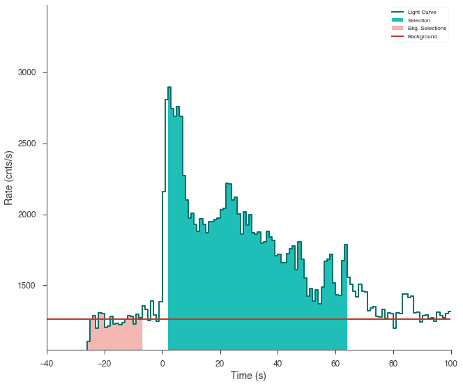
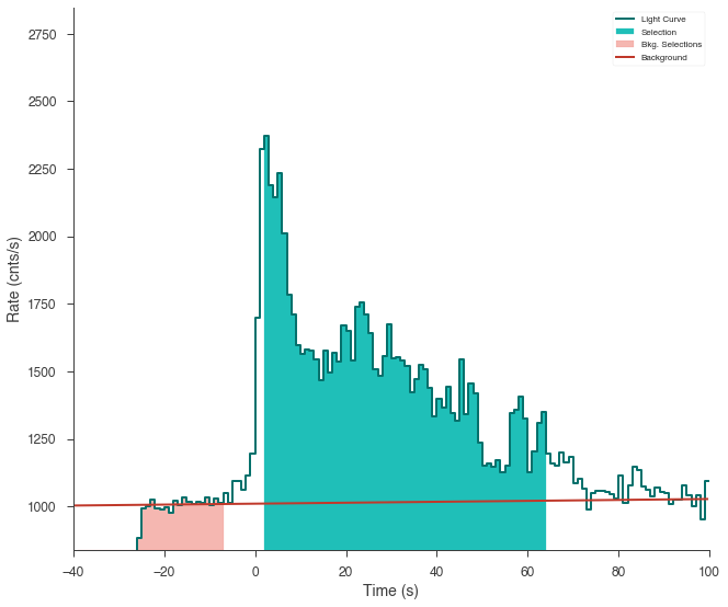
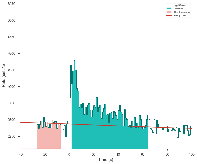
Let’s first examine the catalog fluence fit. Using the TimeSeriesBuilder, we can fit the background, set the source interval, and create a 3ML plugin for the analysis. We will loop through the detectors, set their appropriate channel selections, and ensure there are enough counts in each bin to make the PGStat profile likelihood valid.

• First we use the CSPEC data to fit the background using the background selections. We use CSPEC because it has a longer duration for fitting the background.

• The background is saved to an HDF5 file that stores the polynomial coefficients and selections which we can read in to the TTE file later.

• The light curve is plotted.

• The source selection from the catalog is set and DispersionSpectrumLike plugin is created.

• The plugin has the standard GBM channel selections for spectral analysis set.

fluence_plugins = []
time_series = {}
for det in gbm_detectors:

    ts_cspec = TimeSeriesBuilder.from_gbm_cspec_or_ctime(
        det, cspec_or_ctime_file=dload[det]["cspec"], rsp_file=dload[det]["rsp"]
    )

    ts_cspec.set_background_interval(*background_interval.split(","))
    ts_cspec.save_background(f"{det}_bkg.h5", overwrite=True)

    ts_tte = TimeSeriesBuilder.from_gbm_tte(
        det,
        tte_file=dload[det]["tte"],
        rsp_file=dload[det]["rsp"],
        restore_background=f"{det}_bkg.h5",
    )

    time_series[det] = ts_tte

    ts_tte.set_active_time_interval(source_interval)

    ts_tte.view_lightcurve(-40, 100)

    fluence_plugin = ts_tte.to_spectrumlike()

    if det.startswith("b"):

        fluence_plugin.set_active_measurements("250-30000")

    else:

        fluence_plugin.set_active_measurements("9-900")

    fluence_plugin.rebin_on_background(1.0)

    fluence_plugins.append(fluence_plugin)

Setting up the fit

Let’s see if we can reproduce the results from the catalog.

Set priors for the model

We will fit the spectrum using Bayesian analysis, so we must set priors on the model parameters.

model.GRB080916009.spectrum.main.shape.alpha.prior = Truncated_gaussian(
    lower_bound=-1.5, upper_bound=1, mu=-1, sigma=0.5
)
model.GRB080916009.spectrum.main.shape.beta.prior = Truncated_gaussian(
    lower_bound=-5, upper_bound=-1.6, mu=-2.25, sigma=0.5
)
model.GRB080916009.spectrum.main.shape.break_energy.prior = Log_normal(mu=2, sigma=1)
model.GRB080916009.spectrum.main.shape.break_energy.bounds = (None, None)
model.GRB080916009.spectrum.main.shape.K.prior = Log_uniform_prior(
    lower_bound=1e-3, upper_bound=1e1
)
model.GRB080916009.spectrum.main.shape.break_scale.prior = Log_uniform_prior(
    lower_bound=1e-4, upper_bound=10
)

Clone the model and setup the Bayesian analysis class

Next, we clone the model we built from the catalog so that we can look at the results later and fit the cloned model. We pass this model and the DataList of the plugins to a BayesianAnalysis class and set the sampler to MultiNest.

new_model = clone_model(model)

bayes = BayesianAnalysis(new_model, DataList(*fluence_plugins))

# share spectrum gives a linear speed up when
# spectrumlike plugins have the same RSP input energies
bayes.set_sampler("multinest", share_spectrum=True)

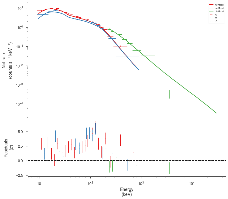
Examine at the catalog fitted model

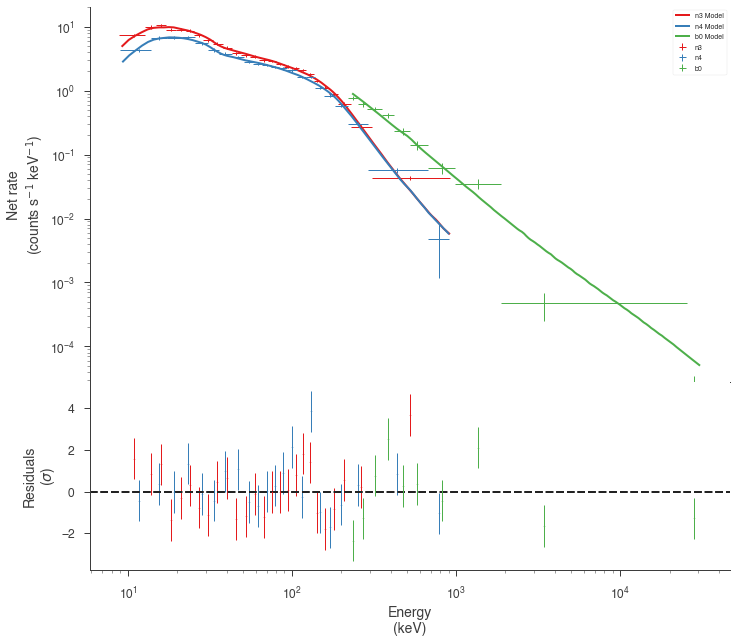
We can quickly examine how well the catalog fit matches the data. There appears to be a discrepancy between the data and the model! Let’s refit to see if we can fix it.

fig = display_spectrum_model_counts(bayes, min_rate=20, step=False)

Run the sampler

We let MultiNest condition the model on the data

bayes.sampler.setup(n_live_points=400)
bayes.sample()

  analysing data from chains/fit-.txt
Maximum a posteriori probability (MAP) point:

	result	unit
parameter
GRB080916009...K	(1.475 -0.019 +0.018) x 10^-2	1 / (cm2 keV s)
GRB080916009...alpha	-1.079 -0.017 +0.016
GRB080916009...break_energy	(2.02 -0.14 +0.15) x 10^2	keV
GRB080916009...break_scale	(1.7 -1.0 +0.8) x 10^-1
GRB080916009...beta	-2.01 +/- 0.05

Values of -log(posterior) at the minimum:

	-log(posterior)
b0	-1049.511750
n3	-1018.831086
n4	-1010.756422
total	-3079.099257

Values of statistical measures:

	statistical measures
AIC	6168.368969
BIC	6187.601179
DIC	6178.065672
PDIC	3.248980
log(Z)	-1347.504951

 *****************************************************
 MultiNest v3.10
 Copyright Farhan Feroz & Mike Hobson
 Release Jul 2015

 no. of live points =  400
 dimensionality =    5
 *****************************************************
 ln(ev)=  -3102.7448138442028      +/-  0.22794185323035443
 Total Likelihood Evaluations:        21744
 Sampling finished. Exiting MultiNest

Now our model seems to match much better with the data!

bayes.restore_median_fit()
fig = display_spectrum_model_counts(bayes, min_rate=20)

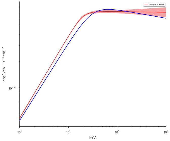
But how different are we from the catalog model? Let’s plot our fit along with the catalog model. Luckily, 3ML can handle all the units for is

conversion = u.Unit("keV2/(cm2 s keV)").to("erg2/(cm2 s keV)")
energy_grid = np.logspace(1, 4, 100) * u.keV
vFv = (energy_grid**2 * model.get_point_source_fluxes(0, energy_grid)).to(
    "erg2/(cm2 s keV)"
)

fig = plot_spectra(bayes.results, flux_unit="erg2/(cm2 s keV)")
ax = fig.get_axes()[0]
_ = ax.loglog(energy_grid, vFv, color="blue", label="catalog model")

Time Resolved Analysis

Now that we have examined fluence fit, we can move to performing a time-resolved analysis.

Selecting a temporal binning

We first get the brightest NaI detector and create time bins via the Bayesian blocks algorithm. We can use the fitted background to make sure that our intervals are chosen in an unbiased way.

n3 = time_series["n3"]

n3.create_time_bins(0, 60, method="bayesblocks", use_background=True, p0=0.2)

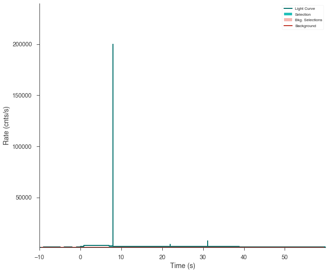
Sometimes, glitches in the GBM data cause spikes in the data that the Bayesian blocks algorithm detects as fast changes in the count rate. We will have to remove those intervals manually.

Note: In the future, 3ML will provide an automated method to remove these unwanted spikes.

fig = n3.view_lightcurve(use_binner=True)

bad_bins = []
for i, w in enumerate(n3.bins.widths):

    if w < 5e-2:
        bad_bins.append(i)


edges = [n3.bins.starts[0]]

for i, b in enumerate(n3.bins):

    if i not in bad_bins:
        edges.append(b.stop)

starts = edges[:-1]
stops = edges[1:]


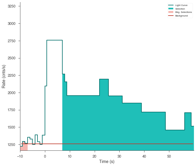
n3.create_time_bins(starts, stops, method="custom")

Now our light curve looks much more acceptable.

fig = n3.view_lightcurve(use_binner=True)

The time series objects can read time bins from each other, so we will map these time bins onto the other detectors’ time series and create a list of time plugins for each detector and each time bin created above.

time_resolved_plugins = {}

for k, v in time_series.items():
    v.read_bins(n3)
    time_resolved_plugins[k] = v.to_spectrumlike(from_bins=True)

Setting up the model

For the time-resolved analysis, we will fit the classic Band function to the data. We will set some principled priors.

band = Band()
band.alpha.prior = Truncated_gaussian(lower_bound=-1.5, upper_bound=1, mu=-1, sigma=0.5)
band.beta.prior = Truncated_gaussian(lower_bound=-5, upper_bound=-1.6, mu=-2, sigma=0.5)
band.xp.prior = Log_normal(mu=2, sigma=1)
band.xp.bounds = (0, None)
band.K.prior = Log_uniform_prior(lower_bound=1e-10, upper_bound=1e3)
ps = PointSource("grb", 0, 0, spectral_shape=band)
band_model = Model(ps)

Perform the fits

One way to perform Bayesian spectral fits to all the intervals is to loop through each one. There can are many ways to do this, so find an analysis pattern that works for you.

models = []
results = []
analysis = []
for interval in range(12):

    # clone the model above so that we have a separate model
    # for each fit

    this_model = clone_model(band_model)

    # for each detector set up the plugin
    # for this time interval

    this_data_list = []
    for k, v in time_resolved_plugins.items():

        pi = v[interval]

        if k.startswith("b"):
            pi.set_active_measurements("250-30000")
        else:
            pi.set_active_measurements("9-900")

        pi.rebin_on_background(1.0)

        this_data_list.append(pi)

    # create a data list

    dlist = DataList(*this_data_list)

    # set up the sampler and fit

    bayes = BayesianAnalysis(this_model, dlist)

    # get some speed with share spectrum
    bayes.set_sampler("multinest", share_spectrum=True)
    bayes.sampler.setup(n_live_points=500)
    bayes.sample()

    # at this stage we coudl also
    # save the analysis result to
    # disk but we will simply hold
    # onto them in memory

    analysis.append(bayes)

  analysing data from chains/fit-.txt
Maximum a posteriori probability (MAP) point:

	result	unit
parameter
grb.spectrum.main.Band.K	(4.14 -0.5 +0.32) x 10^-2	1 / (cm2 keV s)
grb.spectrum.main.Band.alpha	(-5.2 -0.8 +0.7) x 10^-1
grb.spectrum.main.Band.xp	(2.62 -0.30 +0.31) x 10^2	keV
grb.spectrum.main.Band.beta	-1.873 -0.034 +0.07

Values of -log(posterior) at the minimum:

	-log(posterior)
b0_interval0	-286.174296
n3_interval0	-250.047575
n4_interval0	-267.596446
total	-803.818318

Values of statistical measures:

	statistical measures
AIC	1615.749950
BIC	1631.158767
DIC	1570.816989
PDIC	1.980155
log(Z)	-344.067632

  analysing data from chains/fit-.txt
Maximum a posteriori probability (MAP) point:

	result	unit
parameter
grb.spectrum.main.Band.K	(4.30 +/- 0.10) x 10^-2	1 / (cm2 keV s)
grb.spectrum.main.Band.alpha	(-8.29 +/- 0.21) x 10^-1
grb.spectrum.main.Band.xp	(5.59 -0.29 +0.27) x 10^2	keV
grb.spectrum.main.Band.beta	-2.06 +/- 0.06

Values of -log(posterior) at the minimum:

	-log(posterior)
b0_interval1	-674.394248
n3_interval1	-641.475991
n4_interval1	-645.009609
total	-1960.879849

Values of statistical measures:

	statistical measures
AIC	3929.873012
BIC	3945.281829
DIC	3873.723672
PDIC	3.117039
log(Z)	-844.783077

  analysing data from chains/fit-.txt
Maximum a posteriori probability (MAP) point:

	result	unit
parameter
grb.spectrum.main.Band.K	(3.17 -0.22 +0.21) x 10^-2	1 / (cm2 keV s)
grb.spectrum.main.Band.alpha	(-9.2 -0.5 +0.6) x 10^-1
grb.spectrum.main.Band.xp	(3.4 +/- 0.6) x 10^2	keV
grb.spectrum.main.Band.beta	-1.75 +/- 0.08

Values of -log(posterior) at the minimum:

	-log(posterior)
b0_interval2	-323.595653
n3_interval2	-288.125574
n4_interval2	-311.421286
total	-923.142512

Values of statistical measures:

	statistical measures
AIC	1854.398338
BIC	1869.807156
DIC	1806.494927
PDIC	2.288981
log(Z)	-394.775351

  analysing data from chains/fit-.txt
Maximum a posteriori probability (MAP) point:

	result	unit
parameter
grb.spectrum.main.Band.K	(2.9 +/- 0.4) x 10^-2	1 / (cm2 keV s)
grb.spectrum.main.Band.alpha	(-9.3 +/- 1.0) x 10^-1
grb.spectrum.main.Band.xp	(3.6 +/- 0.7) x 10^2	keV
grb.spectrum.main.Band.beta	-2.38 -0.32 +0.33

Values of -log(posterior) at the minimum:

	-log(posterior)
b0_interval3	-298.399604
n3_interval3	-242.503127
n4_interval3	-262.494709
total	-803.397439

Values of statistical measures:

	statistical measures
AIC	1614.908193
BIC	1630.317010
DIC	1571.208881
PDIC	3.268725
log(Z)	-342.142933

  analysing data from chains/fit-.txt
Maximum a posteriori probability (MAP) point:

	result	unit
parameter
grb.spectrum.main.Band.K	(2.05 +/- 0.11) x 10^-2	1 / (cm2 keV s)
grb.spectrum.main.Band.alpha	(-9.8 +/- 0.4) x 10^-1
grb.spectrum.main.Band.xp	(4.1 +/- 0.5) x 10^2	keV
grb.spectrum.main.Band.beta	-2.00 -0.11 +0.10

Values of -log(posterior) at the minimum:

	-log(posterior)
b0_interval4	-778.392672
n3_interval4	-757.099439
n4_interval4	-746.612889
total	-2282.105000

Values of statistical measures:

	statistical measures
AIC	4572.323315
BIC	4587.732133
DIC	4527.878455
PDIC	3.436647
log(Z)	-986.131253

  analysing data from chains/fit-.txt
Maximum a posteriori probability (MAP) point:

	result	unit
parameter
grb.spectrum.main.Band.K	(2.78 -0.19 +0.18) x 10^-2	1 / (cm2 keV s)
grb.spectrum.main.Band.alpha	(-9.2 +/- 0.5) x 10^-1
grb.spectrum.main.Band.xp	(4.4 +/- 0.6) x 10^2	keV
grb.spectrum.main.Band.beta	-2.24 -0.20 +0.19

Values of -log(posterior) at the minimum:

	-log(posterior)
b0_interval5	-537.004055
n3_interval5	-523.488499
n4_interval5	-527.740613
total	-1588.233166

Values of statistical measures:

	statistical measures
AIC	3184.579647
BIC	3199.988464
DIC	3137.076434
PDIC	3.484660
log(Z)	-683.201994

  analysing data from chains/fit-.txt
Maximum a posteriori probability (MAP) point:

	result	unit
parameter
grb.spectrum.main.Band.K	(1.95 -0.12 +0.13) x 10^-2	1 / (cm2 keV s)
grb.spectrum.main.Band.alpha	-1.01 +/- 0.05
grb.spectrum.main.Band.xp	(4.6 +/- 0.7) x 10^2	keV
grb.spectrum.main.Band.beta	-2.49 -0.31 +0.29

Values of -log(posterior) at the minimum:

	-log(posterior)
b0_interval6	-609.552819
n3_interval6	-584.285500
n4_interval6	-576.811753
total	-1770.650071

Values of statistical measures:

	statistical measures
AIC	3549.413457
BIC	3564.822275
DIC	3501.452838
PDIC	3.431436
log(Z)	-762.213471

  analysing data from chains/fit-.txt
Maximum a posteriori probability (MAP) point:

	result	unit
parameter
grb.spectrum.main.Band.K	(1.741 -0.027 +0.026) x 10^-2	1 / (cm2 keV s)
grb.spectrum.main.Band.alpha	-1.116 -0.008 +0.007
grb.spectrum.main.Band.xp	(3.35 -0.15 +0.16) x 10^2	keV
grb.spectrum.main.Band.beta	-1.823 -0.028 +0.020

Values of -log(posterior) at the minimum:

	-log(posterior)
b0_interval7	-665.595430
n3_interval7	-648.785174
n4_interval7	-650.573207
total	-1964.953810

Values of statistical measures:

	statistical measures
AIC	3938.020934
BIC	3953.429751
DIC	3893.301928
PDIC	0.794676
log(Z)	-850.984257

  analysing data from chains/fit-.txt
Maximum a posteriori probability (MAP) point:

	result	unit
parameter
grb.spectrum.main.Band.K	(1.59 -0.14 +0.12) x 10^-2	1 / (cm2 keV s)
grb.spectrum.main.Band.alpha	(-8.3 -0.7 +0.6) x 10^-1
grb.spectrum.main.Band.xp	(3.6 -0.4 +0.5) x 10^2	keV
grb.spectrum.main.Band.beta	-2.13 +/- 0.09

Values of -log(posterior) at the minimum:

	-log(posterior)
b0_interval8	-702.146890
n3_interval8	-698.244472
n4_interval8	-666.350442
total	-2066.741804

Values of statistical measures:

	statistical measures
AIC	4141.596923
BIC	4157.005740
DIC	4097.265832
PDIC	2.568706
log(Z)	-892.686015

  analysing data from chains/fit-.txt
Maximum a posteriori probability (MAP) point:

	result	unit
parameter
grb.spectrum.main.Band.K	(1.5 -0.7 +0.4) x 10^-2	1 / (cm2 keV s)
grb.spectrum.main.Band.alpha	(-8.2 +/- 2.1) x 10^-1
grb.spectrum.main.Band.xp	(1.2 -0.5 +0.4) x 10^2	keV
grb.spectrum.main.Band.beta	-2.10 +/- 0.30

Values of -log(posterior) at the minimum:

	-log(posterior)
b0_interval9	-648.201011
n3_interval9	-617.128654
n4_interval9	-616.478365
total	-1881.808029

Values of statistical measures:

	statistical measures
AIC	3771.729373
BIC	3787.138191
DIC	3699.811876
PDIC	-47.555586
log(Z)	-816.326505

  analysing data from chains/fit-.txt
Maximum a posteriori probability (MAP) point:

	result	unit
parameter
grb.spectrum.main.Band.K	(2.15 -0.4 +0.34) x 10^-2	1 / (cm2 keV s)
grb.spectrum.main.Band.alpha	(-7.3 -1.2 +1.1) x 10^-1
grb.spectrum.main.Band.xp	(2.3 +/- 0.5) x 10^2	keV
grb.spectrum.main.Band.beta	-2.19 -0.32 +0.29

Values of -log(posterior) at the minimum:

	-log(posterior)
b0_interval10	-461.036479
n3_interval10	-437.549891
n4_interval10	-433.425422
total	-1332.011793

Values of statistical measures:

	statistical measures
AIC	2672.136900
BIC	2687.545718
DIC	2634.466592
PDIC	0.738187
log(Z)	-574.275959

  analysing data from chains/fit-.txt
Maximum a posteriori probability (MAP) point:

	result	unit
parameter
grb.spectrum.main.Band.K	(3.8 -1.7 +1.8) x 10^-2	1 / (cm2 keV s)
grb.spectrum.main.Band.alpha	(-4.0 -2.7 +2.9) x 10^-1
grb.spectrum.main.Band.xp	(1.17 -0.24 +0.26) x 10^2	keV
grb.spectrum.main.Band.beta	-2.01 -0.17 +0.19

Values of -log(posterior) at the minimum:

	-log(posterior)
b0_interval11	-292.341443
n3_interval11	-272.312338
n4_interval11	-255.894141
total	-820.547923

Values of statistical measures:

	statistical measures
AIC	1649.209159
BIC	1664.617977
DIC	1616.359841
PDIC	-0.608713
log(Z)	-352.853169

 *****************************************************
 MultiNest v3.10
 Copyright Farhan Feroz & Mike Hobson
 Release Jul 2015

 no. of live points =  500
 dimensionality =    4
 *****************************************************
 ln(ev)=  -792.24500148681591      +/-  0.18983858392512962
 Total Likelihood Evaluations:        17322
 Sampling finished. Exiting MultiNest
 *****************************************************
 MultiNest v3.10
 Copyright Farhan Feroz & Mike Hobson
 Release Jul 2015

 no. of live points =  500
 dimensionality =    4
 *****************************************************
 ln(ev)=  -1945.1849202669891      +/-  0.21660040203748088
 Total Likelihood Evaluations:        22996
 Sampling finished. Exiting MultiNest
 *****************************************************
 MultiNest v3.10
 Copyright Farhan Feroz & Mike Hobson
 Release Jul 2015

 no. of live points =  500
 dimensionality =    4
 *****************************************************
 ln(ev)=  -909.00383751849256      +/-  0.18826936080717696
 Total Likelihood Evaluations:        18754
 Sampling finished. Exiting MultiNest
 *****************************************************
 MultiNest v3.10
 Copyright Farhan Feroz & Mike Hobson
 Release Jul 2015

 no. of live points =  500
 dimensionality =    4
 *****************************************************
 ln(ev)=  -787.81321607490054      +/-  0.17414717671211596
 Total Likelihood Evaluations:        18456
 Sampling finished. Exiting MultiNest
 *****************************************************
 MultiNest v3.10
 Copyright Farhan Feroz & Mike Hobson
 Release Jul 2015

 no. of live points =  500
 dimensionality =    4
 *****************************************************
 ln(ev)=  -2270.6511230658512      +/-  0.19779559737214022
 Total Likelihood Evaluations:        20815
 Sampling finished. Exiting MultiNest
 *****************************************************
 MultiNest v3.10
 Copyright Farhan Feroz & Mike Hobson
 Release Jul 2015

 no. of live points =  500
 dimensionality =    4
 *****************************************************
 ln(ev)=  -1573.1307264488419      +/-  0.19142257925661371
 Total Likelihood Evaluations:        19891
 Sampling finished. Exiting MultiNest
 *****************************************************
 MultiNest v3.10
 Copyright Farhan Feroz & Mike Hobson
 Release Jul 2015

 no. of live points =  500
 dimensionality =    4
 *****************************************************
 ln(ev)=  -1755.0613758706297      +/-  0.19170753325729020
 Total Likelihood Evaluations:        19374
 Sampling finished. Exiting MultiNest
 *****************************************************
 MultiNest v3.10
 Copyright Farhan Feroz & Mike Hobson
 Release Jul 2015

 no. of live points =  500
 dimensionality =    4
 *****************************************************
 ln(ev)=  -1959.4636640781321      +/-  0.21431664030803474
 Total Likelihood Evaluations:        19853
 Sampling finished. Exiting MultiNest
 *****************************************************
 MultiNest v3.10
 Copyright Farhan Feroz & Mike Hobson
 Release Jul 2015

 no. of live points =  500
 dimensionality =    4
 *****************************************************
 ln(ev)=  -2055.4855105210568      +/-  0.19187445620251778
 Total Likelihood Evaluations:        18867
 Sampling finished. Exiting MultiNest
 *****************************************************
 MultiNest v3.10
 Copyright Farhan Feroz & Mike Hobson
 Release Jul 2015

 no. of live points =  500
 dimensionality =    4
 *****************************************************
 ln(ev)=  -1879.6612419007322      +/-  0.15141974690567908
 Total Likelihood Evaluations:        12304
 Sampling finished. Exiting MultiNest
 *****************************************************
 MultiNest v3.10
 Copyright Farhan Feroz & Mike Hobson
 Release Jul 2015

 no. of live points =  500
 dimensionality =    4
 *****************************************************
 ln(ev)=  -1322.3192622534418      +/-  0.16886653621172776
 Total Likelihood Evaluations:        14718
 Sampling finished. Exiting MultiNest
 *****************************************************
 MultiNest v3.10
 Copyright Farhan Feroz & Mike Hobson
 Release Jul 2015

 no. of live points =  500
 dimensionality =    4
 *****************************************************
 ln(ev)=  -812.47444606520730      +/-  0.14849223458898625
 Total Likelihood Evaluations:        12230
 Sampling finished. Exiting MultiNest

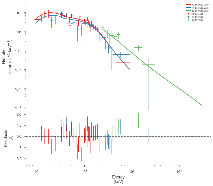
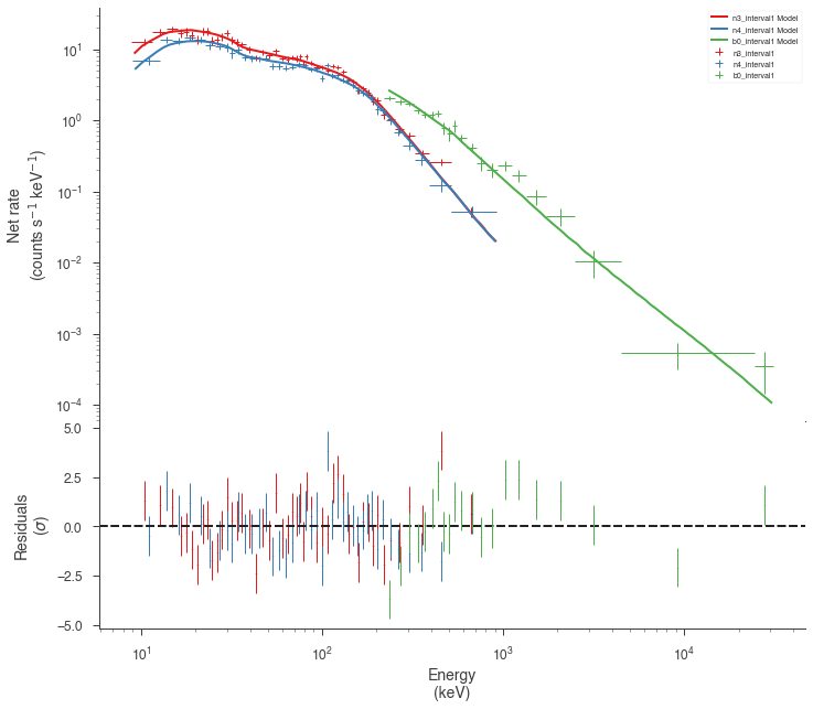
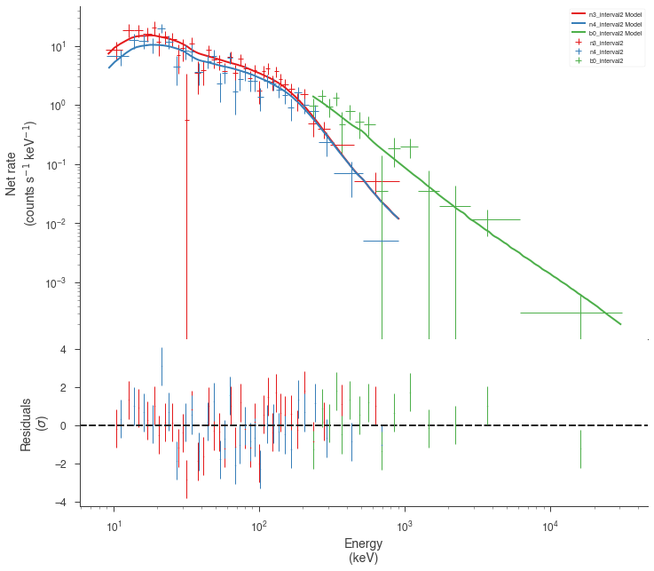
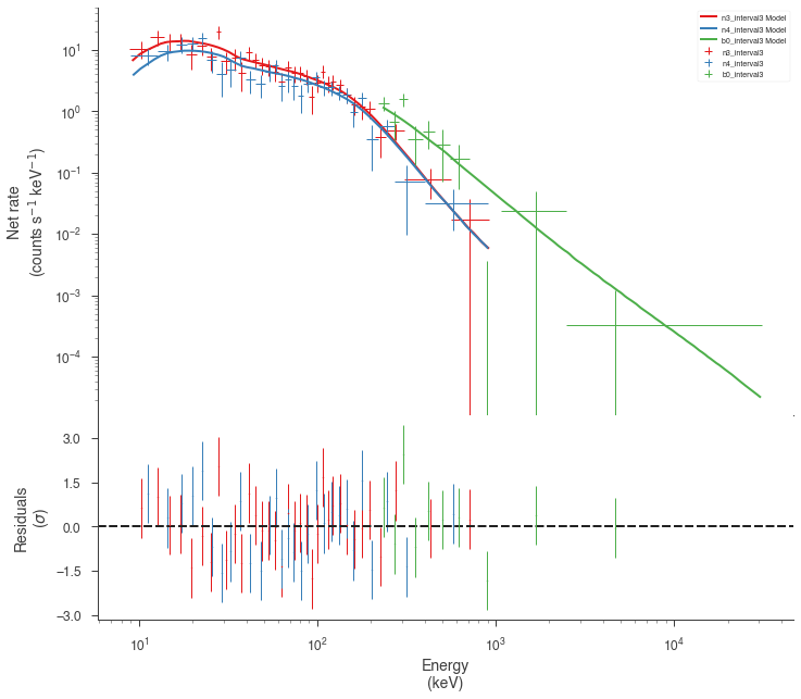
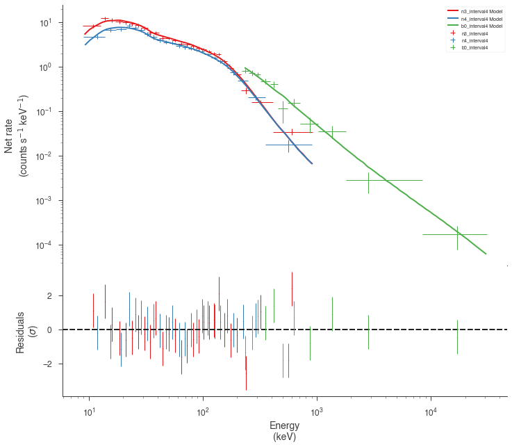
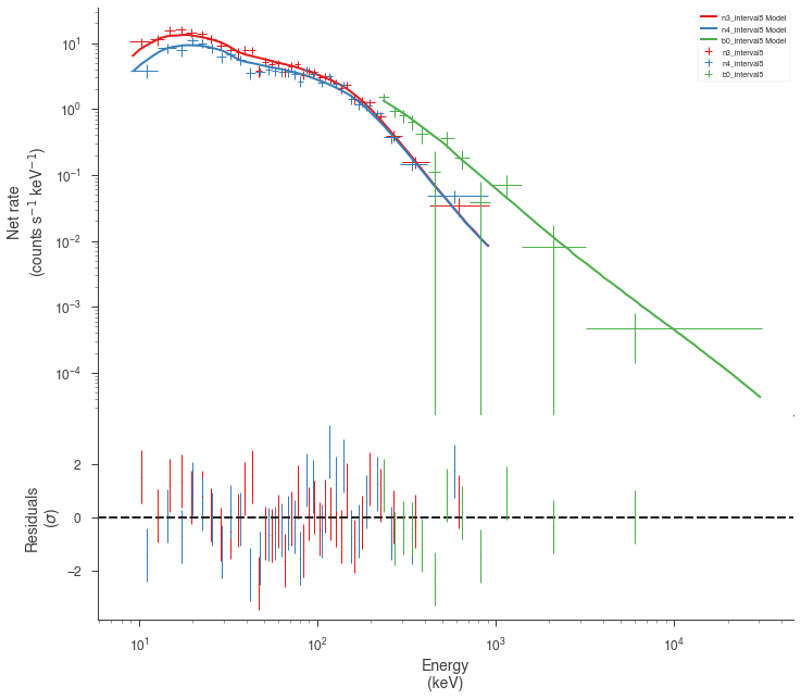
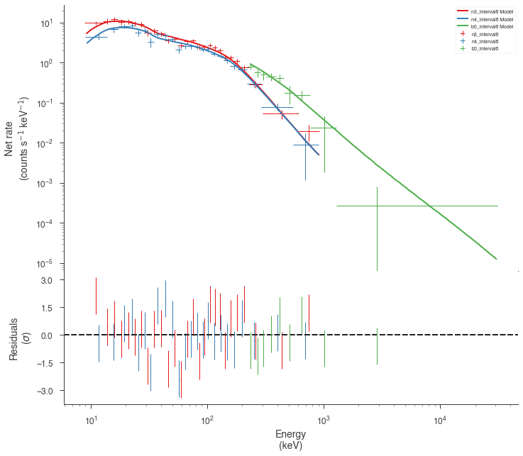
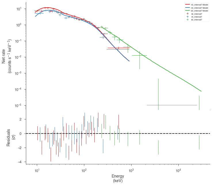
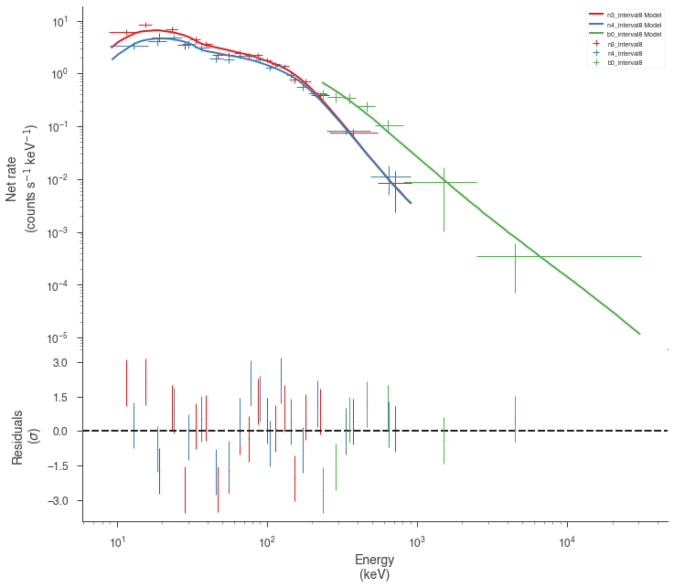
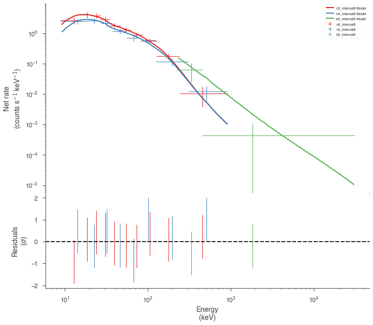
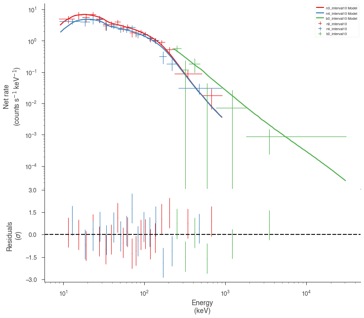
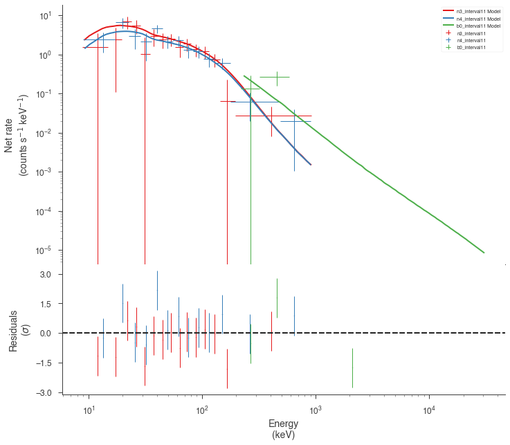
Examine the fits

Now we can look at the fits in count space to make sure they are ok.

for a in analysis:
    a.restore_median_fit()
    _ = display_spectrum_model_counts(a, min_rate=[20, 20, 20], step=False)

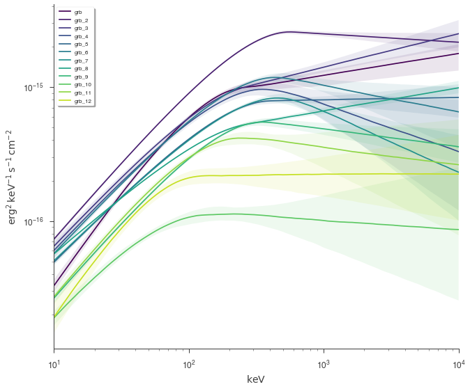
Finally, we can plot the models together to see how the spectra evolve with time.

fig = plot_spectra(
    *[a.results for a in analysis[::1]],
    flux_unit="erg2/(cm2 s keV)",
    fit_cmap="viridis",
    contour_cmap="viridis",
    contour_style_kwargs=dict(alpha=0.1),
)

This example can serve as a template for performing analysis on GBM data. However, as 3ML provides an abstract interface and modular building blocks, similar analysis pipelines can be built for any time series data.