Analyzing GRB 080916C

[Alt text](https://astrobites.org/wp-content/uploads/2014/10/NASAGRBwhoa-1024x576.jpg ” (NASA/Swift/Cruz deWilde)”) (NASA/Swift/Cruz deWilde)

To demonstrate the capabilities and features of 3ML in, we will go through a time-integrated and time-resolved analysis. This example serves as a standard way to analyze Fermi-GBM data with 3ML as well as a template for how you can design your instrument’s analysis pipeline with 3ML if you have similar data.

%%capture
import matplotlib.pyplot as plt
import numpy as np

np.seterr(all="ignore")


from threeML import *
from threeML.io.package_data import get_path_of_data_file

Examining the catalog

As with Swift and Fermi-LAT, 3ML provides a simple interface to the on-line Fermi-GBM catalog. Let’s get the information for GRB 080916C.

gbm_catalog = FermiGBMBurstCatalog()
gbm_catalog.query_sources("GRB080916009")

Table length=1

name	ra	dec	trigger_time	t90
object	float64	float64	float64	float64
GRB080916009	119.800	-56.600	54725.0088613	62.977

To aid in quickly replicating the catalog analysis, and thanks to the tireless efforts of the Fermi-GBM team, we have added the ability to extract the analysis parameters from the catalog as well as build an astromodels model with the best fit parameters baked in. Using this information, one can quickly run through the catalog an replicate the entire analysis with a script. Let’s give it a try.

grb_info = gbm_catalog.get_detector_information()["GRB080916009"]

gbm_detectors = grb_info["detectors"]
source_interval = grb_info["source"]["fluence"]
background_interval = grb_info["background"]["full"]
best_fit_model = grb_info["best fit model"]["fluence"]
model = gbm_catalog.get_model(best_fit_model, "fluence")["GRB080916009"]

model

Model summary:

	N
Point sources	1
Extended sources	0
Particle sources	0

Free parameters (5):

	value	min_value	max_value	unit
GRB080916009.spectrum.main.SmoothlyBrokenPowerLaw.K	0.012255	0.0	None	keV-1 s-1 cm-2
GRB080916009.spectrum.main.SmoothlyBrokenPowerLaw.alpha	-1.130424	-1.5	2.0
GRB080916009.spectrum.main.SmoothlyBrokenPowerLaw.break_energy	309.2031	10.0	None	keV
GRB080916009.spectrum.main.SmoothlyBrokenPowerLaw.break_scale	0.3	0.0	10.0
GRB080916009.spectrum.main.SmoothlyBrokenPowerLaw.beta	-2.096931	-5.0	-1.6

Fixed parameters (3):
(abridged. Use complete=True to see all fixed parameters)


Linked parameters (0):

(none)

Independent variables:

(none)

Downloading the data

We provide a simple interface to download the Fermi-GBM data. Using the information from the catalog that we have extracted, we can download just the data from the detectors that were used for the catalog analysis. This will download the CSPEC, TTE and instrument response files from the on-line database.

dload = download_GBM_trigger_data("bn080916009", detectors=gbm_detectors)

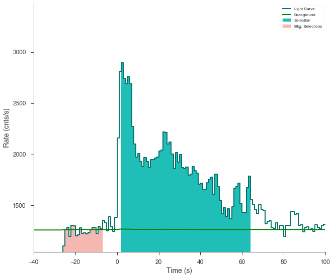
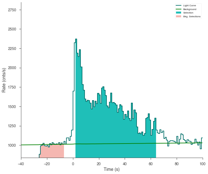
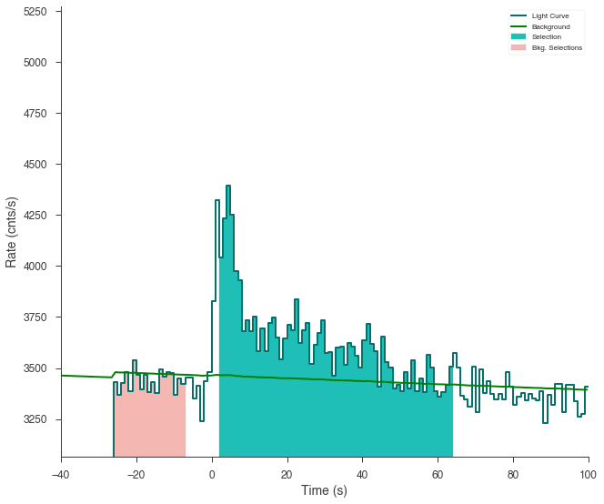
Let’s first examine the catalof fluence fit. Using the TimeSeriesBuilder, we can fit the background, set the source interval, and create a 3ML plugin for the analysis. We will loop through the detectors, set their appropriate channel selections, and ensure there are enough counts in each bin to make the PGStat profile likelihood valid.

• First we use the CSPEC data to fit the background using the background selections. We use CSPEC because it has a longer duration for fitting the background.

• The background is saved to an HDF5 file that stores the polynomial coefficients and selections which we can read in to the TTE file later.

• The light curve is plotted.

• The source selection from the catalog is set and DispersionSpectrumLike plugin is created.

• The plugin has the standard GBM channel selections for spectral analysis set.

fluence_plugins = []
time_series = {}
for det in gbm_detectors:

    ts_cspec = TimeSeriesBuilder.from_gbm_cspec_or_ctime(
        det, cspec_or_ctime_file=dload[det]["cspec"], rsp_file=dload[det]["rsp"]
    )

    ts_cspec.set_background_interval(*background_interval.split(","))
    ts_cspec.save_background(f"{det}_bkg.h5", overwrite=True)

    ts_tte = TimeSeriesBuilder.from_gbm_tte(
        det,
        tte_file=dload[det]["tte"],
        rsp_file=dload[det]["rsp"],
        restore_background=f"{det}_bkg.h5",
    )

    time_series[det] = ts_tte

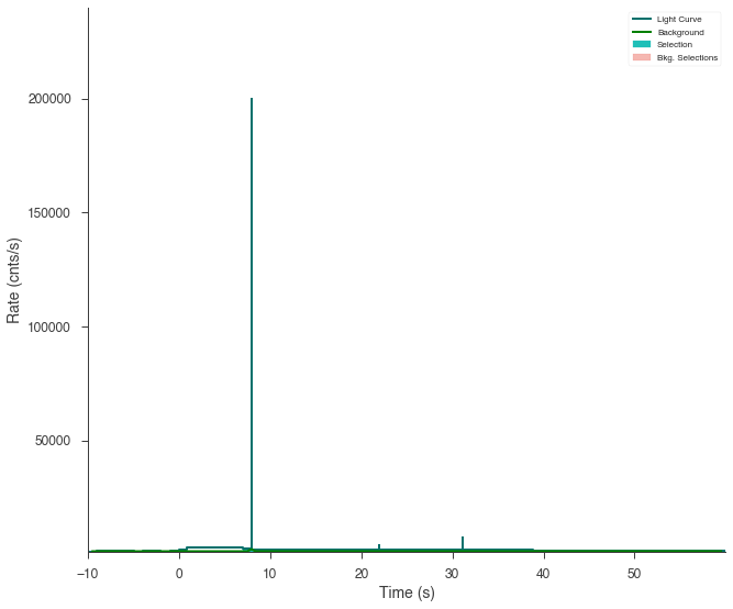
    ts_tte.set_active_time_interval(source_interval)

    ts_tte.view_lightcurve(-40, 100)

    fluence_plugin = ts_tte.to_spectrumlike()

    if det.startswith("b"):

        fluence_plugin.set_active_measurements("250-30000")

    else:

        fluence_plugin.set_active_measurements("9-900")

    fluence_plugin.rebin_on_background(1.0)

    fluence_plugins.append(fluence_plugin)

Setting up the fit

Let’s see if we can reproduce the results from the catalog.

Set priors for the model

We will fit the spectrum using Bayesian analysis, so we must set priors on the model parameters.

model.GRB080916009.spectrum.main.shape.alpha.prior = Truncated_gaussian(
    lower_bound=-1.5, upper_bound=1, mu=-1, sigma=0.5
)
model.GRB080916009.spectrum.main.shape.beta.prior = Truncated_gaussian(
    lower_bound=-5, upper_bound=-1.6, mu=-2.25, sigma=0.5
)
model.GRB080916009.spectrum.main.shape.break_energy.prior = Log_normal(mu=2, sigma=1)
model.GRB080916009.spectrum.main.shape.break_energy.bounds = (None, None)
model.GRB080916009.spectrum.main.shape.K.prior = Log_uniform_prior(
    lower_bound=1e-3, upper_bound=1e1
)
model.GRB080916009.spectrum.main.shape.break_scale.prior = Log_uniform_prior(
    lower_bound=1e-4, upper_bound=10
)

Clone the model and setup the Bayesian analysis class

Next, we clone the model we built from the catalog so that we can look at the results later and fit the cloned model. We pass this model and the DataList of the plugins to a BayesianAnalysis class and set the sampler to MultiNest.

new_model = clone_model(model)

bayes = BayesianAnalysis(new_model, DataList(*fluence_plugins))

# share spectrum gives a linear speed up when
# spectrumlike plugins have the same RSP input energies
bayes.set_sampler("multinest", share_spectrum=True)

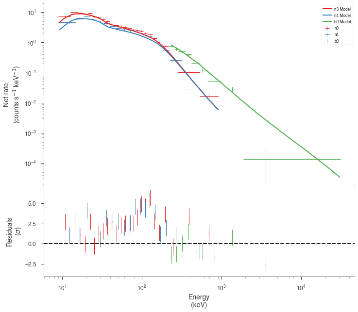
Examine at the catalog fitted model

We can quickly examine how well the catalog fit matches the data. There appears to be a discrepancy between the data and the model! Let’s refit to see if we can fix it.

fig = display_spectrum_model_counts(bayes, min_rate=20, step=False)

Run the sampler

We let MultiNest condition the model on the data

bayes.sampler.setup(n_live_points=400)
bayes.sample()

  analysing data from chains/fit-.txt
Maximum a posteriori probability (MAP) point:

	result	unit
parameter
GRB080916009...K	(1.472 -0.018 +0.019) x 10^-2	1 / (cm2 keV s)
GRB080916009...alpha	-1.072 -0.017 +0.018
GRB080916009...break_energy	(2.17 -0.24 +0.23) x 10^2	keV
GRB080916009...break_scale	(2.0 +/- 0.8) x 10^-1
GRB080916009...beta	-2.12 -0.09 +0.08

Values of -log(posterior) at the minimum:

	-log(posterior)
b0	-1052.132137
n3	-1022.818197
n4	-1014.716152
total	-3089.666485

Values of statistical measures:

	statistical measures
AIC	6189.503425
BIC	6208.735635
DIC	6176.121235
PDIC	4.277981
log(Z)	-1347.848966

 *****************************************************
 MultiNest v3.10
 Copyright Farhan Feroz & Mike Hobson
 Release Jul 2015

 no. of live points =  400
 dimensionality =    5
 *****************************************************
 ln(ev)=  -3103.5369362739448      +/-  0.22489296753381510
 Total Likelihood Evaluations:        22849
 Sampling finished. Exiting MultiNest

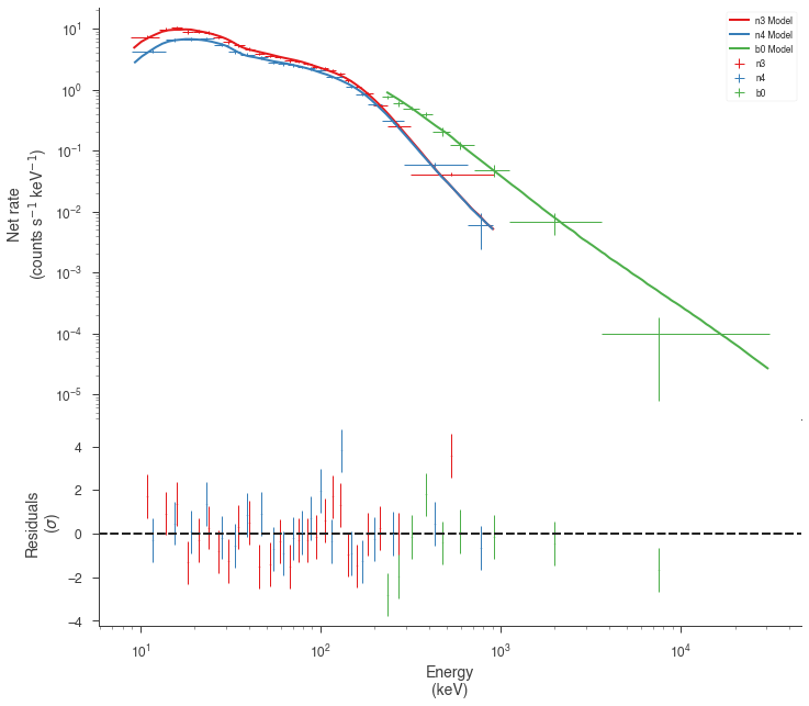
Now our model seems to match much better with the data!

bayes.restore_median_fit()
fig = display_spectrum_model_counts(bayes, min_rate=20)

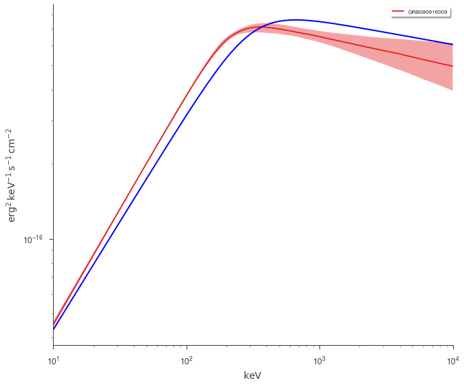
But how different are we from the catalog model? Let’s plot our fit along with the catalog model. Luckily, 3ML can handle all the units for is

conversion = u.Unit("keV2/(cm2 s keV)").to("erg2/(cm2 s keV)")
energy_grid = np.logspace(1, 4, 100) * u.keV
vFv = (energy_grid ** 2 * model.get_point_source_fluxes(0, energy_grid)).to(
    "erg2/(cm2 s keV)"
)

fig = plot_spectra(bayes.results, flux_unit="erg2/(cm2 s keV)")
ax = fig.get_axes()[0]
_ = ax.loglog(energy_grid, vFv, color="blue", label="catalog model")

Time Resolved Analysis

Now that we have examined fluence fit, we can move to performing a time-resolved analysis.

Selecting a temporal binning

We first get the brightest NaI detector and create time bins via the Bayesian blocks algorithm. We can use the fitted background to make sure that our intervals are chosen in an unbiased way.

n3 = time_series["n3"]

n3.create_time_bins(0, 60, method="bayesblocks", use_background=True, p0=0.2)

Sometimes, glitches in the GBM data cause spikes in the data that the Bayesian blocks algorithm detects as fast changes in the count rate. We will have to remove those intervals manually.

...note In the future, 3ML will provide an automated method to remove these unwanted spikes.

fig = n3.view_lightcurve(use_binner=True)

bad_bins = []
for i, w in enumerate(n3.bins.widths):

    if w < 5e-2:
        bad_bins.append(i)


edges = [n3.bins.starts[0]]

for i, b in enumerate(n3.bins):

    if i not in bad_bins:
        edges.append(b.stop)

starts = edges[:-1]
stops = edges[1:]


n3.create_time_bins(starts, stops, method="custom")

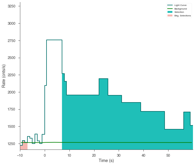
Now our light curve looks much more acceptable.

fig = n3.view_lightcurve(use_binner=True)

The time series objects can read time bins from each other, so we will map these time bins onto the other detectors’ time series and create a list of time plugins for each detector and each time bin created above.

time_resolved_plugins = {}

for k, v in time_series.items():
    v.read_bins(n3)
    time_resolved_plugins[k] = v.to_spectrumlike(from_bins=True)

Setting up the model

For the time-resolved analysis, we will fit the classic Band function to the data. We will set some principled priors.

band = Band()
band.alpha.prior = Truncated_gaussian(lower_bound=-1.5, upper_bound=1, mu=-1, sigma=0.5)
band.beta.prior = Truncated_gaussian(lower_bound=-5, upper_bound=-1.6, mu=-2, sigma=0.5)
band.xp.prior = Log_normal(mu=2, sigma=1)
band.xp.bounds = (0, None)
band.K.prior = Log_uniform_prior(lower_bound=1e-10, upper_bound=1e3)
ps = PointSource("grb", 0, 0, spectral_shape=band)
band_model = Model(ps)

Perform the fits

One way to perform Bayesian spectral fits to all the intervals is to loop through each one. There can are many ways to do this, so find an analysis pattern that works for you.

models = []
results = []
analysis = []
for interval in range(12):

    # clone the model above so that we have a separate model
    # for each fit

    this_model = clone_model(band_model)

    # for each detector set up the plugin
    # for this time interval

    this_data_list = []
    for k, v in time_resolved_plugins.items():

        pi = v[interval]

        if k.startswith("b"):
            pi.set_active_measurements("250-30000")
        else:
            pi.set_active_measurements("9-900")

        pi.rebin_on_background(1.0)

        this_data_list.append(pi)

    # create a data list

    dlist = DataList(*this_data_list)

    # set up the sampler and fit

    bayes = BayesianAnalysis(this_model, dlist)

    # get some speed with share spectrum
    bayes.set_sampler("multinest", share_spectrum=True)
    bayes.sampler.setup(n_live_points=500)
    bayes.sample()

    # at this stage we coudl also
    # save the analysis result to
    # disk but we will simply hold
    # onto them in memory

    analysis.append(bayes)

  analysing data from chains/fit-.txt
Maximum a posteriori probability (MAP) point:

	result	unit
parameter
grb.spectrum.main.Band.K	(3.5 +/- 0.6) x 10^-2	1 / (cm2 keV s)
grb.spectrum.main.Band.alpha	(-5.6 -1.4 +1.3) x 10^-1
grb.spectrum.main.Band.xp	(3.4 +/- 0.6) x 10^2	keV
grb.spectrum.main.Band.beta	-2.25 +/- 0.29

Values of -log(posterior) at the minimum:

	-log(posterior)
b0_interval0	-280.518424
n3_interval0	-245.222926
n4_interval0	-261.484826
total	-787.226176

Values of statistical measures:

	statistical measures
AIC	1582.565667
BIC	1597.974484
DIC	1560.889553
PDIC	2.534274
log(Z)	-342.885089

  analysing data from chains/fit-.txt
Maximum a posteriori probability (MAP) point:

	result	unit
parameter
grb.spectrum.main.Band.K	(5.16 -0.11 +0.10) x 10^-2	1 / (cm2 keV s)
grb.spectrum.main.Band.alpha	(-6.81 -0.14 +0.15) x 10^-1
grb.spectrum.main.Band.xp	(3.81 -0.09 +0.08) x 10^2	keV
grb.spectrum.main.Band.beta	-1.889 -0.022 +0.023

Values of -log(posterior) at the minimum:

	-log(posterior)
b0_interval1	-674.361978
n3_interval1	-639.007003
n4_interval1	-637.491699
total	-1950.860680

Values of statistical measures:

	statistical measures
AIC	3909.834674
BIC	3925.243491
DIC	3889.797474
PDIC	2.527368
log(Z)	-852.557983

  analysing data from chains/fit-.txt
Maximum a posteriori probability (MAP) point:

	result	unit
parameter
grb.spectrum.main.Band.K	(2.45 +/- 0.19) x 10^-2	1 / (cm2 keV s)
grb.spectrum.main.Band.alpha	-1.07 +/- 0.06
grb.spectrum.main.Band.xp	(7.3 +/- 1.8) x 10^2	keV
grb.spectrum.main.Band.beta	-2.61 +/- 0.31

Values of -log(posterior) at the minimum:

	-log(posterior)
b0_interval2	-317.234383
n3_interval2	-283.400752
n4_interval2	-306.296277
total	-906.931413

Values of statistical measures:

	statistical measures
AIC	1821.976140
BIC	1837.384957
DIC	1792.323094
PDIC	3.256983
log(Z)	-393.719089

  analysing data from chains/fit-.txt
Maximum a posteriori probability (MAP) point:

	result	unit
parameter
grb.spectrum.main.Band.K	(2.95 -0.24 +0.25) x 10^-2	1 / (cm2 keV s)
grb.spectrum.main.Band.alpha	(-9.2 -0.8 +0.7) x 10^-1
grb.spectrum.main.Band.xp	(3.4 +/- 0.5) x 10^2	keV
grb.spectrum.main.Band.beta	-2.66 -0.24 +0.23

Values of -log(posterior) at the minimum:

	-log(posterior)
b0_interval3	-292.051353
n3_interval3	-237.309056
n4_interval3	-257.355419
total	-786.715828

Values of statistical measures:

	statistical measures
AIC	1581.544971
BIC	1596.953789
DIC	1558.077737
PDIC	2.237529
log(Z)	-343.079008

  analysing data from chains/fit-.txt
Maximum a posteriori probability (MAP) point:

	result	unit
parameter
grb.spectrum.main.Band.K	(2.10 -0.14 +0.11) x 10^-2	1 / (cm2 keV s)
grb.spectrum.main.Band.alpha	(-9.6 +/- 0.4) x 10^-1
grb.spectrum.main.Band.xp	(3.9 -0.5 +0.6) x 10^2	keV
grb.spectrum.main.Band.beta	-2.09 +/- 0.15

Values of -log(posterior) at the minimum:

	-log(posterior)
b0_interval4	-773.394015
n3_interval4	-751.447512
n4_interval4	-741.134708
total	-2265.976235

Values of statistical measures:

	statistical measures
AIC	4540.065784
BIC	4555.474601
DIC	4520.649450
PDIC	3.348748
log(Z)	-987.310146

  analysing data from chains/fit-.txt
Maximum a posteriori probability (MAP) point:

	result	unit
parameter
grb.spectrum.main.Band.K	(3.32 -0.10 +0.14) x 10^-2	1 / (cm2 keV s)
grb.spectrum.main.Band.alpha	(-8.34 -0.18 +0.29) x 10^-1
grb.spectrum.main.Band.xp	(2.82 -0.19 +0.18) x 10^2	keV
grb.spectrum.main.Band.beta	-1.746 -0.013 +0.012

Values of -log(posterior) at the minimum:

	-log(posterior)
b0_interval5	-539.355030
n3_interval5	-518.096672
n4_interval5	-524.347765
total	-1581.799466

Values of statistical measures:

	statistical measures
AIC	3171.712246
BIC	3187.121064
DIC	3152.428181
PDIC	1.456402
log(Z)	-692.313021

  analysing data from chains/fit-.txt
Maximum a posteriori probability (MAP) point:

	result	unit
parameter
grb.spectrum.main.Band.K	(2.00 +/- 0.11) x 10^-2	1 / (cm2 keV s)
grb.spectrum.main.Band.alpha	(-9.9 +/- 0.4) x 10^-1
grb.spectrum.main.Band.xp	(4.2 +/- 0.5) x 10^2	keV
grb.spectrum.main.Band.beta	-2.55 +/- 0.31

Values of -log(posterior) at the minimum:

	-log(posterior)
b0_interval6	-607.134535
n3_interval6	-577.813971
n4_interval6	-570.940458
total	-1755.888964

Values of statistical measures:

	statistical measures
AIC	3519.891242
BIC	3535.300060
DIC	3496.886197
PDIC	3.251197
log(Z)	-764.437768

  analysing data from chains/fit-.txt
Maximum a posteriori probability (MAP) point:

	result	unit
parameter
grb.spectrum.main.Band.K	(1.68 -0.11 +0.10) x 10^-2	1 / (cm2 keV s)
grb.spectrum.main.Band.alpha	-1.03 +/- 0.05
grb.spectrum.main.Band.xp	(4.3 +/- 0.6) x 10^2	keV
grb.spectrum.main.Band.beta	-2.52 -0.29 +0.28

Values of -log(posterior) at the minimum:

	-log(posterior)
b0_interval7	-659.385228
n3_interval7	-634.946260
n4_interval7	-644.643311
total	-1938.974798

Values of statistical measures:

	statistical measures
AIC	3886.062911
BIC	3901.471729
DIC	3863.981720
PDIC	3.377095
log(Z)	-843.849787

  analysing data from chains/fit-.txt
Maximum a posteriori probability (MAP) point:

	result	unit
parameter
grb.spectrum.main.Band.K	(1.83 -0.10 +0.09) x 10^-2	1 / (cm2 keV s)
grb.spectrum.main.Band.alpha	(-7.8 -0.4 +0.5) x 10^-1
grb.spectrum.main.Band.xp	(2.53 -0.13 +0.15) x 10^2	keV
grb.spectrum.main.Band.beta	-1.796 -0.025 +0.029

Values of -log(posterior) at the minimum:

	-log(posterior)
b0_interval8	-701.361814
n3_interval8	-695.470634
n4_interval8	-662.437905
total	-2059.270352

Values of statistical measures:

	statistical measures
AIC	4126.654019
BIC	4142.062837
DIC	4111.594361
PDIC	2.036232
log(Z)	-899.790594

  analysing data from chains/fit-.txt
Maximum a posteriori probability (MAP) point:

	result	unit
parameter
grb.spectrum.main.Band.K	(1.5 -0.7 +0.6) x 10^-2	1 / (cm2 keV s)
grb.spectrum.main.Band.alpha	(-7.8 -2.3 +2.4) x 10^-1
grb.spectrum.main.Band.xp	(1.2 +/- 0.4) x 10^2	keV
grb.spectrum.main.Band.beta	-2.08 -0.28 +0.27

Values of -log(posterior) at the minimum:

	-log(posterior)
b0_interval9	-647.027712
n3_interval9	-615.118430
n4_interval9	-613.663494
total	-1875.809635

Values of statistical measures:

	statistical measures
AIC	3759.732585
BIC	3775.141403
DIC	3729.144703
PDIC	-16.413692
log(Z)	-816.824300

  analysing data from chains/fit-.txt
Maximum a posteriori probability (MAP) point:

	result	unit
parameter
grb.spectrum.main.Band.K	(2.2 -0.5 +0.4) x 10^-2	1 / (cm2 keV s)
grb.spectrum.main.Band.alpha	(-7.1 -1.3 +1.4) x 10^-1
grb.spectrum.main.Band.xp	(2.2 +/- 0.5) x 10^2	keV
grb.spectrum.main.Band.beta	-2.23 -0.32 +0.34

Values of -log(posterior) at the minimum:

	-log(posterior)
b0_interval10	-457.171674
n3_interval10	-433.999601
n4_interval10	-428.974014
total	-1320.145289

Values of statistical measures:

	statistical measures
AIC	2648.403892
BIC	2663.812709
DIC	2630.368313
PDIC	1.397418
log(Z)	-575.185713

  analysing data from chains/fit-.txt
Maximum a posteriori probability (MAP) point:

	result	unit
parameter
grb.spectrum.main.Band.K	(3.2 +/- 1.3) x 10^-2	1 / (cm2 keV s)
grb.spectrum.main.Band.alpha	(-4.7 -2.4 +2.5) x 10^-1
grb.spectrum.main.Band.xp	(1.33 -0.29 +0.30) x 10^2	keV
grb.spectrum.main.Band.beta	-2.32 -0.35 +0.33

Values of -log(posterior) at the minimum:

	-log(posterior)
b0_interval11	-289.621967
n3_interval11	-268.876265
n4_interval11	-252.593074
total	-811.091306

Values of statistical measures:

	statistical measures
AIC	1630.295926
BIC	1645.704743
DIC	1612.260414
PDIC	-0.114767
log(Z)	-353.503653

 *****************************************************
 MultiNest v3.10
 Copyright Farhan Feroz & Mike Hobson
 Release Jul 2015

 no. of live points =  500
 dimensionality =    4
 *****************************************************
 ln(ev)=  -789.52209348829319      +/-  0.17474889251418757
 Total Likelihood Evaluations:        17080
 Sampling finished. Exiting MultiNest
 *****************************************************
 MultiNest v3.10
 Copyright Farhan Feroz & Mike Hobson
 Release Jul 2015

 no. of live points =  500
 dimensionality =    4
 *****************************************************
 ln(ev)=  -1963.0873035486127      +/-  0.22178035725874823
 Total Likelihood Evaluations:        23669
 Sampling finished. Exiting MultiNest
 *****************************************************
 MultiNest v3.10
 Copyright Farhan Feroz & Mike Hobson
 Release Jul 2015

 no. of live points =  500
 dimensionality =    4
 *****************************************************
 ln(ev)=  -906.57170455673952      +/-  0.19308160782910277
 Total Likelihood Evaluations:        24834
 Sampling finished. Exiting MultiNest
 *****************************************************
 MultiNest v3.10
 Copyright Farhan Feroz & Mike Hobson
 Release Jul 2015

 no. of live points =  500
 dimensionality =    4
 *****************************************************
 ln(ev)=  -789.96860935235770      +/-  0.18469927133768616
 Total Likelihood Evaluations:        16701
 Sampling finished. Exiting MultiNest
 *****************************************************
 MultiNest v3.10
 Copyright Farhan Feroz & Mike Hobson
 Release Jul 2015

 no. of live points =  500
 dimensionality =    4
 *****************************************************
 ln(ev)=  -2273.3656241309136      +/-  0.19716513304781941
 Total Likelihood Evaluations:        20343
 Sampling finished. Exiting MultiNest
 *****************************************************
 MultiNest v3.10
 Copyright Farhan Feroz & Mike Hobson
 Release Jul 2015

 no. of live points =  500
 dimensionality =    4
 *****************************************************
 ln(ev)=  -1594.1096408135945      +/-  0.21419111411854921
 Total Likelihood Evaluations:        20341
 Sampling finished. Exiting MultiNest
 *****************************************************
 MultiNest v3.10
 Copyright Farhan Feroz & Mike Hobson
 Release Jul 2015

 no. of live points =  500
 dimensionality =    4
 *****************************************************
 ln(ev)=  -1760.1830099588944      +/-  0.19285814240574450
 Total Likelihood Evaluations:        20598
 Sampling finished. Exiting MultiNest
 *****************************************************
 MultiNest v3.10
 Copyright Farhan Feroz & Mike Hobson
 Release Jul 2015

 no. of live points =  500
 dimensionality =    4
 *****************************************************
 ln(ev)=  -1943.0359393711108      +/-  0.18898932905297527
 Total Likelihood Evaluations:        21829
 Sampling finished. Exiting MultiNest
 *****************************************************
 MultiNest v3.10
 Copyright Farhan Feroz & Mike Hobson
 Release Jul 2015

 no. of live points =  500
 dimensionality =    4
 *****************************************************
 ln(ev)=  -2071.8444076703950      +/-  0.20453050984780796
 Total Likelihood Evaluations:        20080
 Sampling finished. Exiting MultiNest
 *****************************************************
 MultiNest v3.10
 Copyright Farhan Feroz & Mike Hobson
 Release Jul 2015

 no. of live points =  500
 dimensionality =    4
 *****************************************************
 ln(ev)=  -1880.8074573100555      +/-  0.14395400075906434
 Total Likelihood Evaluations:        12903
 Sampling finished. Exiting MultiNest
 *****************************************************
 MultiNest v3.10
 Copyright Farhan Feroz & Mike Hobson
 Release Jul 2015

 no. of live points =  500
 dimensionality =    4
 *****************************************************
 ln(ev)=  -1324.4140479273581      +/-  0.16580877676791583
 Total Likelihood Evaluations:        15178
 Sampling finished. Exiting MultiNest
 *****************************************************
 MultiNest v3.10
 Copyright Farhan Feroz & Mike Hobson
 Release Jul 2015

 no. of live points =  500
 dimensionality =    4
 *****************************************************
 ln(ev)=  -813.97224143628068      +/-  0.14850585526194979
 Total Likelihood Evaluations:        12133
 Sampling finished. Exiting MultiNest

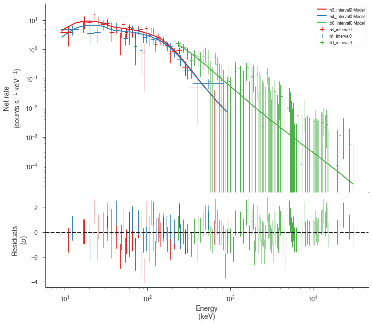
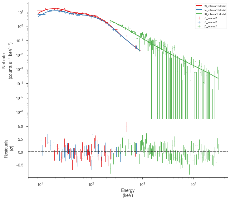
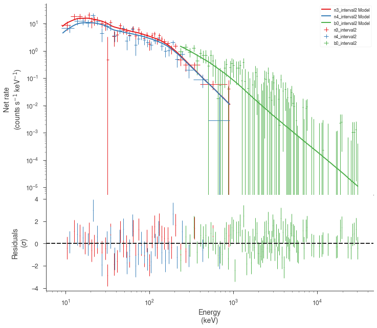
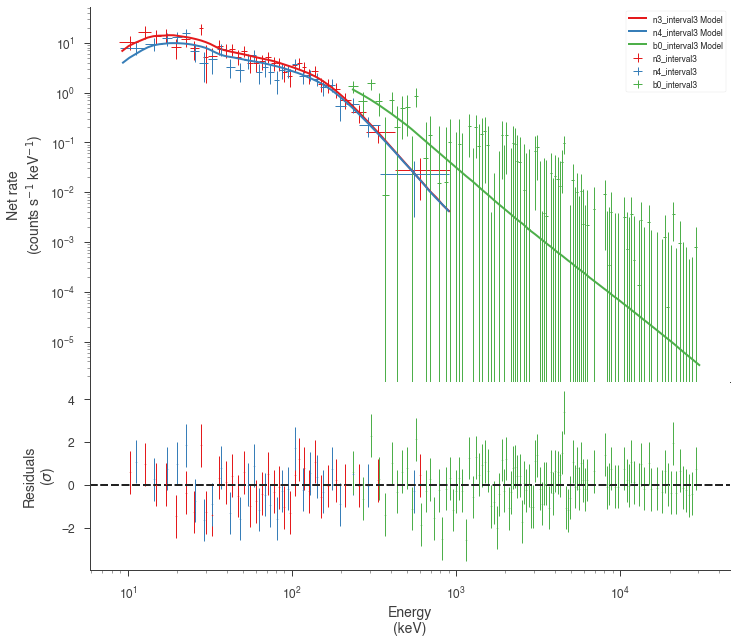
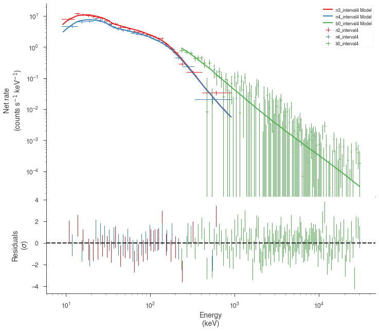
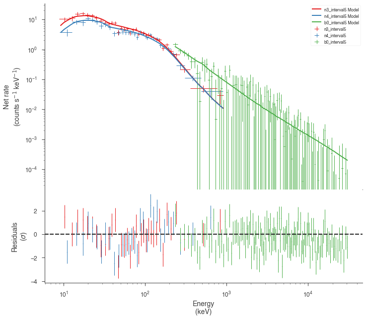
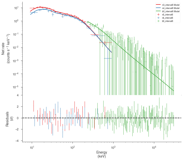
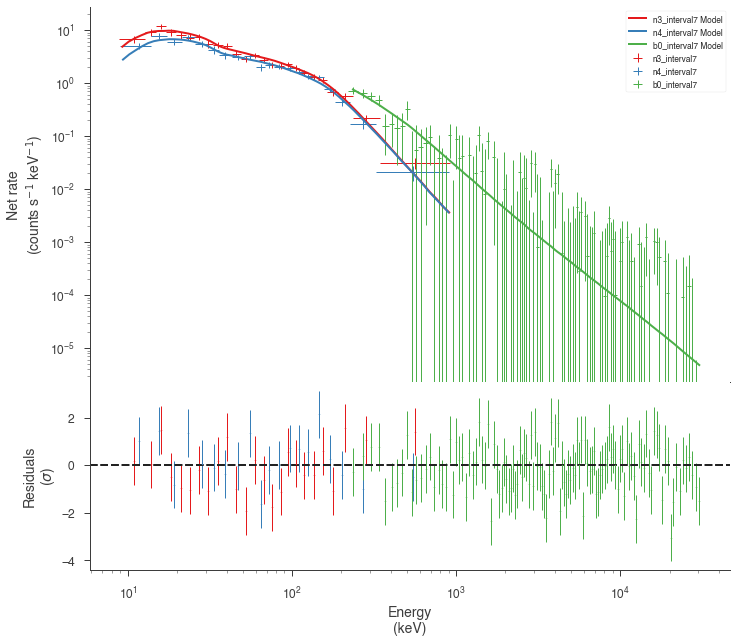
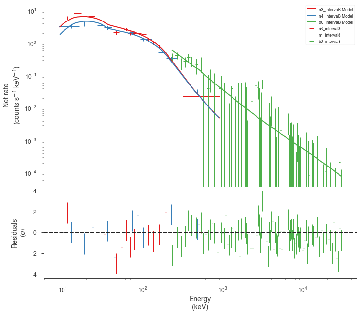
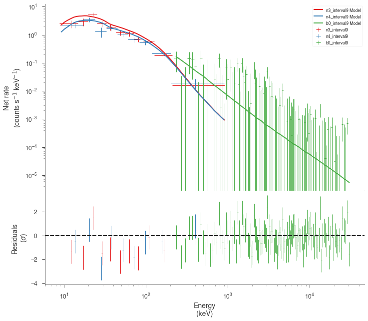
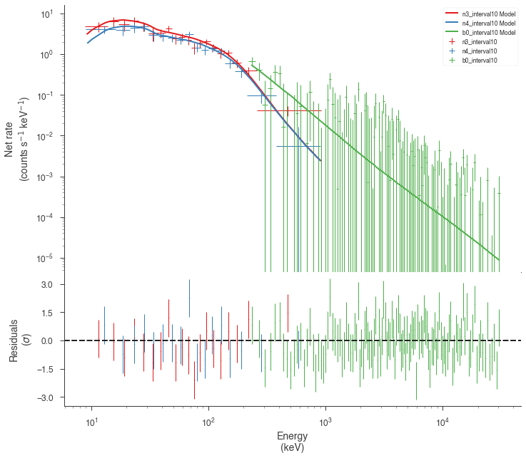
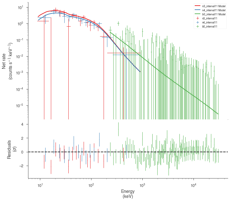
Examine the fits

Now we can look at the fits in count space to make sure they are ok.

for a in analysis:
    a.restore_median_fit()
    _ = display_spectrum_model_counts(a, min_rate=[20, 20, -99], step=False)

Finally, we can plot the models together to see how the spectra evolve with time.

fig = plot_spectra(
    *[a.results for a in analysis[::1]],
    flux_unit="erg2/(cm2 s keV)",
    fit_cmap="viridis",
    contour_cmap="viridis",
    contour_style_kwargs=dict(alpha=0.1),
)

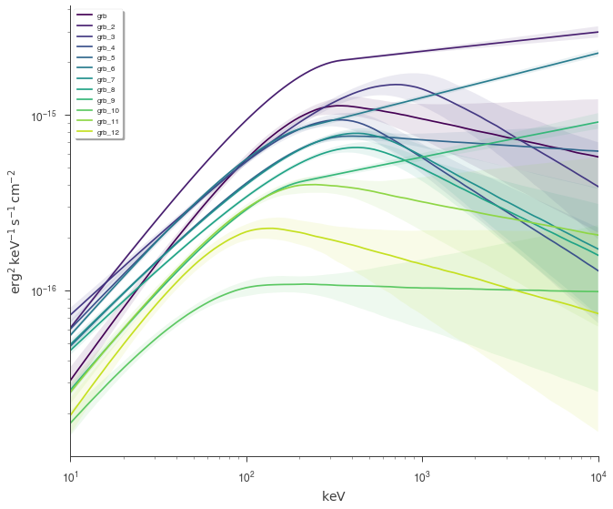
This example can serve as a template for performing analysis on GBM data. However, as 3ML provides an abstract interface and modular building blocks, similar analysis pipelines can be built for any time series data.