HAL (HAWC Accelerated Likelihood) plugin

The High-Altitude Water Cherenkov Observatory (HAWC) is a ground-based wide-field TeV gamma-ray observatory located in Mexico, scanning about 2/3 of the northern sky every day. It is sensitive to gamma rays in the energy range from hundreds of GeV to hundreds of TeV. In addition to gamma ray-induced air showers, HAWC also detects signals from cosmic-ray induced air showers, which make up the main (and partially irreducible) background. HAWC uses a forward-folding likelihood analysis, similar to the approach that is used e.g. by many Fermi-LAT analyses. Most of HAWC’s data are only available to collaboration members. However, HAWC has released several partial-sky datasets to the public, and is committed to releasing more in the future. If you are interested in a particular HAWC dataset, you can find contact information for HAWC working group leaders on the linked webpage.

The HAL (HAWC accelerated likelihood) plugin for threeML is provided in a separate python package, hawc_hal. Before running this example offline, make sure that the HAL plugin is installed. The hawc_hal package needs root_numpy as a dependency. It can be installed as follows (skip the first step if you already have threeML/astromodels installed):

conda create -y --name hal_env -c conda-forge -c threeml numpy scipy matplotlib ipython numba reproject "astromodels>=2" "threeml>=2" root
conda activate hal_env
pip install --no-binary :all: root_numpy
pip install git+https://github.com/threeml/hawc_hal.git

Download

First, download the 507 day Crab dataset and instrument response file from the HAWC webpage. In case of problems with the code below, the files can be downloaded manually from https://data.hawc-observatory.org/datasets/crab_data/index.php . If the files already exist, the code won’t try to overwrite them.

import requests
import shutil
import os

def get_hawc_file( filename, odir = "./", overwrite = False ):

    if overwrite or not os.path.exists( odir + filename):
        url="https://data.hawc-observatory.org/datasets/crab_data/public_data/crab_2017/"

        req = requests.get(url+filename, verify=False,stream=True)
        req.raw.decode_content = True
        with open( odir + filename, 'wb') as f:
            shutil.copyfileobj(r.raw, f)

    return odir + filename


maptree = "HAWC_9bin_507days_crab_data.hd5"
response = "HAWC_9bin_507days_crab_response.hd5"
odir = "./"


maptree = get_hawc_file(maptree, odir)
response = get_hawc_file(response, odir)

assert( os.path.exists(maptree))
assert( os.path.exists(response))

Next, we need to define the region of interest (ROI) and instantiate the HAL plugin. The provided data file is a partial map covering 3˚ around the nominal position of the Crab nebula, so we need to make sure we use the same ROI (or a subset) here.

Some parameters of note:

flat_sky_pixels_size=0.1: HAWC data is provided in counts binned according to the HealPIX scheme, with NSIDE=1024. To reduce computing time, the HAL plugin performs the convolution of the model with the detector response on a rectangular grid on the plane tangent to the center of the ROI. The convolved counts are finally converted back to HealPIX for the calculation of the likelihood. The parameter flat_sky_pixel_size of the HAL class controls the size of the grid used in the convolution with the detector response. Larger grid spacing reduced computing time, but can make the results less reliable. The grid spacing should not be significantly larger than the HealPix pixel size. Also note that model features smaller than the grid spacing may not contribute to the convolved source image. The default here is 0.1˚

hawc.set_active_measurements(1, 9): HAWC divides its data in general analysis bins, each labeled with a string. The dataset provided here uses 9 bins labeled with integers from 1 to 9 and binned according to the fraction of PMTs hit by a particular shower, which is correlated to the energy of the primary particle. See Abeysekara et al., 2017 for details about the meaning of the bins. There are two ways to set the ‘active’ bins (bins to be considered for the fit) in the HAL plugin: set_active_measurement(bin_id_min=1, bin_id_max=9) (can only be used with numerical bins) and set_active_measurement(bin_list=[1,2,3,4,5,6,7,8,9]).

from hawc_hal import HAL, HealpixConeROI
import matplotlib.pyplot as plt
from threeML import *

# Define the ROI.
ra_crab, dec_crab = 83.63,22.02
data_radius = 3.0 #in degree
model_radius = 8.0 #in degree

roi = HealpixConeROI(data_radius=data_radius,
                     model_radius=model_radius,
                     ra=ra_crab,
                     dec=dec_crab)

# Instance the plugin
hawc = HAL("HAWC",
           maptree,
           response,
           roi,
           flat_sky_pixels_size=0.1)

# Use from bin 1 to bin 9
hawc.set_active_measurements(1, 9)

Welcome to JupyROOT 6.22/02

WARNING UserWarning: Using default configuration from /Users/hfleisc1/opt/anaconda3/envs/st3ml/lib/python3.7/site-packages/threeML/data/threeML_config.yml. You might want to copy it to /Users/hfleisc1/.threeML/threeML_config.yml to customize it and avoid this warning.


WARNING RuntimeWarning: numpy.ufunc size changed, may indicate binary incompatibility. Expected 192 from C header, got 216 from PyObject


WARNING RuntimeWarning: numpy.ufunc size changed, may indicate binary incompatibility. Expected 192 from C header, got 216 from PyObject


WARNING RuntimeWarning: numpy.ufunc size changed, may indicate binary incompatibility. Expected 192 from C header, got 216 from PyObject


WARNING RuntimeWarning: Env. variable OMP_NUM_THREADS is not set. Please set it to 1 for optimal performances in 3ML


WARNING RuntimeWarning: Env. variable MKL_NUM_THREADS is not set. Please set it to 1 for optimal performances in 3ML


WARNING RuntimeWarning: Env. variable NUMEXPR_NUM_THREADS is not set. Please set it to 1 for optimal performances in 3ML


WARNING RuntimeWarning: numpy.ufunc size changed, may indicate binary incompatibility. Expected 192 from C header, got 216 from PyObject

Creating singleton for /Users/hfleisc1/hawc_software/my3ML/3ML/docs/notebooks/HAWC_9bin_507days_crab_response.hd5

Exploratory analysis

Next, let’s explore the HAWC data.

First, print some information about the ROI and the data:

hawc.display()

Region of Interest:
-------------------

HealpixConeROI: Center (R.A., Dec) = (83.630, 22.020), data radius = 3.000 deg, model radius: 8.000 deg

Flat sky projection:
--------------------

Width x height: 160 x 160 px
Pixel sizes: 0.1 deg

Response:
---------

Response file: /Users/hfleisc1/hawc_software/my3ML/3ML/docs/notebooks/HAWC_9bin_507days_crab_response.hd5
Number of dec bins: 101
Number of energy/nHit planes per dec bin_name: 9

Map Tree:
----------

	Bin	Nside	Scheme	Obs counts	Bkg counts	obs/bkg	Pixels in ROI	Area (deg^2)
0	0	1024	RING	450572866.0	4.504941e+08	1.000175	8629	28.290097
1	1	1024	RING	31550239.0	3.150819e+07	1.001335	8629	28.290097
2	2	1024	RING	10080669.0	1.005106e+07	1.002945	8629	28.290097
3	3	1024	RING	2737051.0	2.721557e+06	1.005693	8629	28.290097
4	4	1024	RING	346666.0	3.400225e+05	1.019538	8629	28.290097
5	5	1024	RING	77507.0	7.437867e+04	1.042060	8629	28.290097
6	6	1024	RING	14141.0	1.321418e+04	1.070139	8629	28.290097
7	7	1024	RING	8279.0	7.735450e+03	1.070267	8629	28.290097
8	8	1024	RING	2240.0	2.047489e+03	1.094023	8629	28.290097
9	9	1024	RING	3189.0	2.950479e+03	1.080842	8629	28.290097

This Map Tree contains 508.195 transits in the first bin
Total data size: 1.38 Mb

Active energy/nHit planes (9):
-------------------------------

['1', '2', '3', '4', '5', '6', '7', '8', '9']

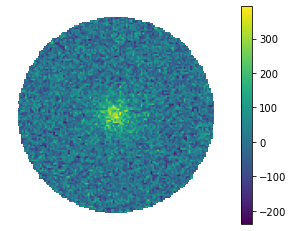
Next, some plots. We can use the display_stacked_image() function to visualize the background-subtracted counts, summed over all (active) bins. This function smoothes the counts for plotting and takes the width of the smoothing kernel as an argument. This width must be non-zero.

First, let’s see what the counts look like without (or very little) smoothing:

%matplotlib inline
fig = hawc.display_stacked_image(smoothing_kernel_sigma=0.01)

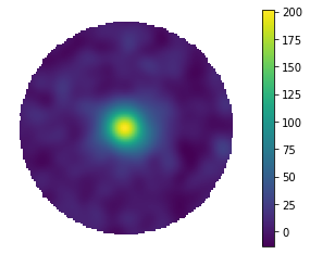
What about smoothing it with a smoothing kernel comparable to the PSF? (Note the change in the color scale!)

fig_smooth = hawc.display_stacked_image(smoothing_kernel_sigma=0.2)

Now, let’s see how the data change from bin to bin (feel free to play around with the smoothing radius here)!

for bin in [1, 5, 9]:

    #set only one active bin
    hawc.set_active_measurements(bin, bin)

    fig = hawc.display_stacked_image(smoothing_kernel_sigma=0.01)
    fig.suptitle("Bin {}".format(bin))

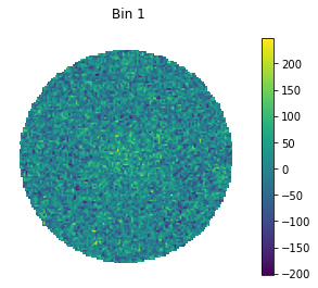
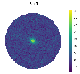
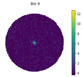
Smaller bins have more events overall, but also more background, and a larger PSF.

Simple model fit

Let’s set up a simple one-source model with a log-parabolic spectrum. For now, the source position will be fixed to its nominal position.

# Define model
spectrum = Log_parabola()
source = PointSource("crab", ra=ra_crab, dec=dec_crab, spectral_shape=spectrum)

spectrum.piv = 7 * u.TeV
spectrum.piv.fix = True

spectrum.K = 1e-14 / (u.TeV * u.cm ** 2 * u.s)  # norm (in 1/(TeV cm2 s))
spectrum.K.bounds = (1e-35, 1e-10) / (u.TeV * u.cm ** 2 * u.s)  # without units energies would be in keV

spectrum.alpha = -2.5  # log parabolic alpha (index)
spectrum.alpha.bounds = (-4., 2.)

spectrum.beta = 0  # log parabolic beta (curvature)
spectrum.beta.bounds = (-1., 1.)

model = Model(source)

model.display(complete=True)

WARNING UserWarning: We have set the min_value of crab.spectrum.main.Log_parabola.K to 1e-99 because there was a postive transform

Model summary:

	N
Point sources	1
Extended sources	0
Particle sources	0

Free parameters (3):

	value	min_value	max_value	unit
crab.spectrum.main.Log_parabola.K	1e-23	1e-44	1e-19	keV-1 s-1 cm-2
crab.spectrum.main.Log_parabola.alpha	-2.5	-4	2
crab.spectrum.main.Log_parabola.beta	0	-1	1

Fixed parameters (3):

	value	min_value	max_value	unit
crab.position.ra	83.63	0	360	deg
crab.position.dec	22.02	-90	90	deg
crab.spectrum.main.Log_parabola.piv	7e+09	None	None	keV

Linked parameters (0):

(none)

Independent variables:

(none)

Next, set up the likelihood object and run the fit. Fit results are written to disk so they can be read in again later.

#make sure to re-set the active bins before the fit
hawc.set_active_measurements(1, 9)
data = DataList(hawc)

jl = JointLikelihood(model, data, verbose=False)
jl.set_minimizer("minuit")
param_df, like_df = jl.fit()

results=jl.results
results.write_to("crab_lp_public_results.fits", overwrite=True)
results.optimized_model.save("crab_fit.yml", overwrite=True)

WARNING RuntimeWarning: numpy.ufunc size changed, may indicate binary incompatibility. Expected 192 from C header, got 216 from PyObject

Best fit values:

	result	unit
parameter
crab.spectrum.main.Log_parabola.K	(2.54 +/- 0.06) x 10^-22	1 / (cm2 keV s)
crab.spectrum.main.Log_parabola.alpha	-2.646 +/- 0.018
crab.spectrum.main.Log_parabola.beta	(1.04 +/- 0.14) x 10^-1

Correlation matrix:

1.00	-0.07	0.82
-0.07	1.00	-0.39
0.82	-0.39	1.00

Values of -log(likelihood) at the minimum:

	-log(likelihood)
HAWC	18765.836788
total	18765.836788

Values of statistical measures:

	statistical measures
AIC	37537.673854
BIC	37565.769982

Assessing the Fit Quality

HAL and threeML provide several ways to assess the quality of the provided model, both quantitatively and qualitatively.

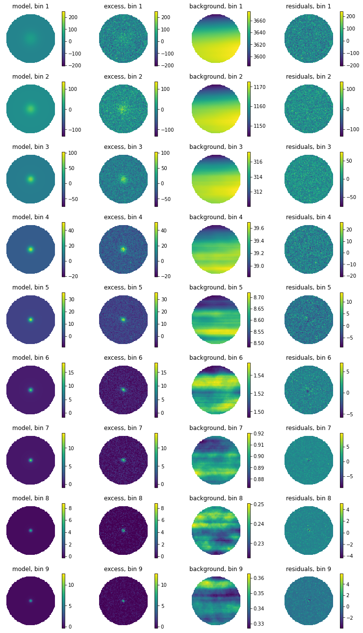
For a first visual impression, we can display the model, excess (counts - background), background, and residuals (counts - model - background) for each bin.

fig = hawc.display_fit(smoothing_kernel_sigma=0.01,display_colorbar=True)

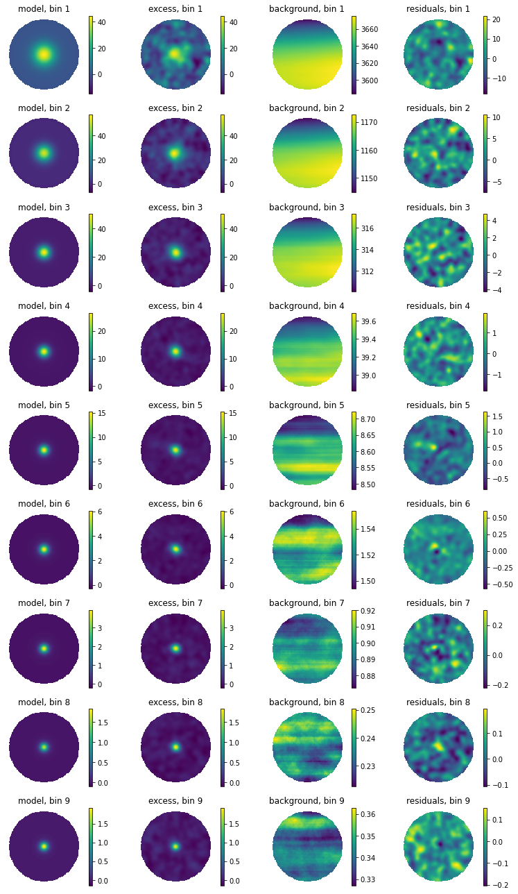
Same, but with smoothing:

fig = hawc.display_fit(smoothing_kernel_sigma=0.2,display_colorbar=True)

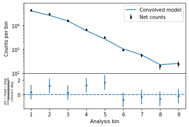
The following plot provides a summary of the images above:

fig = hawc.display_spectrum()

WARNING MatplotlibDeprecationWarning: The 'nonposy' parameter of __init__() has been renamed 'nonpositive' since Matplotlib 3.3; support for the old name will be dropped two minor releases later.

The GoodnessOfFit module provides a numerical assessment of the goodness of fit, by comparing the best-fit likelihood from the fit to likelihood values seen in “simulated” data (background + source model + pseudo-random poissonian fluctuation).

gof_obj = GoodnessOfFit(jl)
gof, data_frame, like_data_frame = gof_obj.by_mc(n_iterations=200)

p = gof["total"]

print("Goodness of fit (p-value:)", p)
print("Meaning that {:.1f}% of simulations have a larger (worse) likelihood".format(100*p) )
print("and {:.1f}% of simulations have a smaller (better) likelihood than seen in data".format(100*(1-p) ) )

df = like_data_frame.reset_index()
df = df[df.level_1 == "total"]

fig, ax = plt.subplots()
ax.hist(df["-log(likelihood)"], label = "fluctuated source models", bins=range(18000,19000,50))
ax.axvline(like_df.loc["total","-log(likelihood)"], label = "fit to data", color = "orange" )
ax.xlabel = "-log(likelihood)"
ax.legend(loc="best")

Goodness of fit (p-value:) 0.1
Meaning that 10.0% of simulations have a larger (worse) likelihood
and 90.0% of simulations have a smaller (better) likelihood than seen in data

<matplotlib.legend.Legend at 0x7fd2ad1cf590>

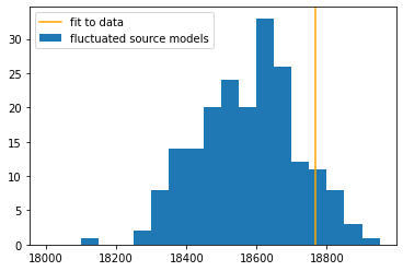
Not too bad, but not great 🙃. The model might be improved by freeing the position or choosing another spectral shape. However, note that the detector response file provided here is the one used in the 2017 publication, which has since been superceeded by an updated detector model (only available inside the HAWC collaboration for now). Discrepancies between the simulated and true detector response may also worsen the goodness of fit.

Visualizing the Fit Results

Now that we have satisfied ourselves that the best-fit model describes the data reasonably well, let’s look at the fit parameters. First, let’s print them again:

param_df

	value	negative_error	positive_error	error	unit
crab.spectrum.main.Log_parabola.K	2.540438e-22	-6.365929e-24	6.168854e-24	6.267392e-24	1 / (cm2 keV s)
crab.spectrum.main.Log_parabola.alpha	-2.645944e+00	-1.765481e-02	1.796397e-02	1.780939e-02
crab.spectrum.main.Log_parabola.beta	1.038799e-01	-1.449745e-02	1.378226e-02	1.413985e-02

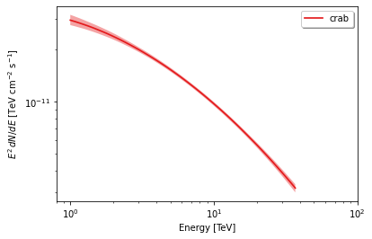
Plot the spectrum using threeML’s plot_spectra convenience function:

fig, ax = plt.subplots()

plot_spectra(results,
                   ene_min=1.0,
                   ene_max=37,
                   num_ene=50,
                   energy_unit='TeV',
                   flux_unit='TeV/(s cm2)',
                   subplot = ax)
ax.set_xlim(0.8,100)
ax.set_ylabel(r"$E^2\,dN/dE$ [TeV cm$^{-2}$ s$^{-1}$]")
ax.set_xlabel("Energy [TeV]")

Text(0.5, 0, 'Energy [TeV]')

What about visualizing the fit parameter’s uncertainties and their correlations? We can use likelihood profiles for that. We need to provide the range for the contours. We can derive a reasonable range from the best-fit values and their uncertainties.

range_min = {}
range_max = {}

params = model.free_parameters
N_param = len(model.free_parameters.keys() )

for name in params:
    row = param_df.loc[name]
    range_min[name] = row["value"] + 5*row["negative_error"]
    range_max[name] = row["value"] + 5*row["positive_error"]

for i in range(0,N_param):
    p1 = list(params.keys())[i]
    p2 = list(params.keys())[(i+1)%N_param]

    a, b, cc, fig = jl.get_contours(p1, range_min[p1], range_max[p1], 20,
                                p2, range_min[p2], range_max[p2], 20 )

WARNING MatplotlibDeprecationWarning: You are modifying the state of a globally registered colormap. In future versions, you will not be able to modify a registered colormap in-place. To remove this warning, you can make a copy of the colormap first. cmap = copy.copy(mpl.cm.get_cmap("Pastel1"))


WARNING MatplotlibDeprecationWarning: You are modifying the state of a globally registered colormap. In future versions, you will not be able to modify a registered colormap in-place. To remove this warning, you can make a copy of the colormap first. cmap = copy.copy(mpl.cm.get_cmap("Pastel1"))


WARNING MatplotlibDeprecationWarning: You are modifying the state of a globally registered colormap. In future versions, you will not be able to modify a registered colormap in-place. To remove this warning, you can make a copy of the colormap first. cmap = copy.copy(mpl.cm.get_cmap("Pastel1"))

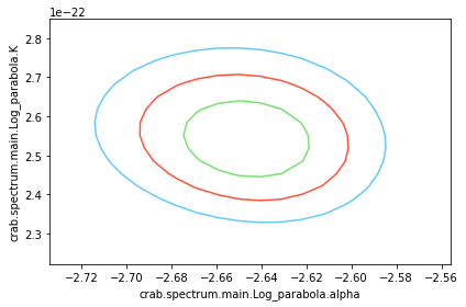
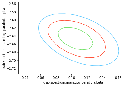
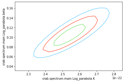
We can see that the index and normalization are essentially uncorrelated (as the pivot energy was chosen accordingly). There is significant correlation between the spectral index and the curvature parameter though.