Analyzing GRB 080916C with Fermi-GBM
 (NASA/Swift/Cruz deWilde)
To demonstrate the capabilities and features of 3ML in, we will go through a time-integrated and time-resolved analysis. This example serves as a standard way to analyze Fermi-GBM data with 3ML as well as a template for how you can design your instrument’s analysis pipeline with 3ML if you have similar data.
3ML provides utilities to reduce time series data to plugins in a correct and statistically justified way (e.g., background fitting of Poisson data is done with a Poisson likelihood). The approach is generic and can be extended. For more details, see the time series documentation.
[1]:
import warnings

warnings.simplefilter("ignore")
[2]:
%%capture
import matplotlib.pyplot as plt
import numpy as np

np.seterr(all="ignore")


from threeML import *
from threeML.io.package_data import get_path_of_data_file
[3]:
silence_warnings()
%matplotlib inline
from jupyterthemes import jtplot

jtplot.style(context="talk", fscale=1, ticks=True, grid=False)
set_threeML_style()
Examining the catalog
As with Swift and Fermi-LAT, 3ML provides a simple interface to the on-line Fermi-GBM catalog. Let’s get the information for GRB 080916C.
[4]:
gbm_catalog = FermiGBMBurstCatalog()
gbm_catalog.query_sources("GRB080916009")
23:25:52 INFO      The cache for fermigbrst does not yet exist. We will try to    get_heasarc_table_as_pandas.py:63
                  build it
INFO Building cache for fermigbrst get_heasarc_table_as_pandas.py:103
[4]:
| name | ra | dec | trigger_time | t90 |
|---|---|---|---|---|
| object | float64 | float64 | float64 | float64 |
| GRB080916009 | 119.800 | -56.600 | 54725.0088613 | 62.977 |
To aid in quickly replicating the catalog analysis, and thanks to the tireless efforts of the Fermi-GBM team, we have added the ability to extract the analysis parameters from the catalog as well as build an astromodels model with the best fit parameters baked in. Using this information, one can quickly run through the catalog an replicate the entire analysis with a script. Let’s give it a try.
[5]:
grb_info = gbm_catalog.get_detector_information()["GRB080916009"]

gbm_detectors = grb_info["detectors"]
source_interval = grb_info["source"]["fluence"]
background_interval = grb_info["background"]["full"]
best_fit_model = grb_info["best fit model"]["fluence"]
model = gbm_catalog.get_model(best_fit_model, "fluence")["GRB080916009"]
[6]:
model
[6]:
| N | |
|---|---|
| Point sources | 1 |
| Extended sources | 0 |
| Particle sources | 0 |
Free parameters (5):
| value | min_value | max_value | unit | |
|---|---|---|---|---|
| GRB080916009.spectrum.main.SmoothlyBrokenPowerLaw.K | 0.012255 | 0.0 | None | keV-1 s-1 cm-2 |
| GRB080916009.spectrum.main.SmoothlyBrokenPowerLaw.alpha | -1.130424 | -1.5 | 2.0 | |
| GRB080916009.spectrum.main.SmoothlyBrokenPowerLaw.break_energy | 309.2031 | 10.0 | None | keV |
| GRB080916009.spectrum.main.SmoothlyBrokenPowerLaw.break_scale | 0.3 | 0.0 | 10.0 | |
| GRB080916009.spectrum.main.SmoothlyBrokenPowerLaw.beta | -2.096931 | -5.0 | -1.6 |
Fixed parameters (3):
(abridged. Use complete=True to see all fixed parameters)
Properties (0):
(none)
Linked parameters (0):
(none)
Independent variables:
(none)
Linked functions (0):
(none)
Downloading the data
We provide a simple interface to download the Fermi-GBM data. Using the information from the catalog that we have extracted, we can download just the data from the detectors that were used for the catalog analysis. This will download the CSPEC, TTE and instrument response files from the on-line database.
[7]:
dload = download_GBM_trigger_data("bn080916009", detectors=gbm_detectors)
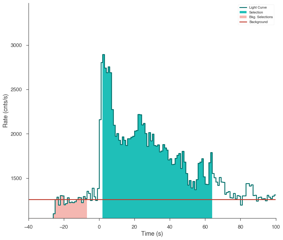
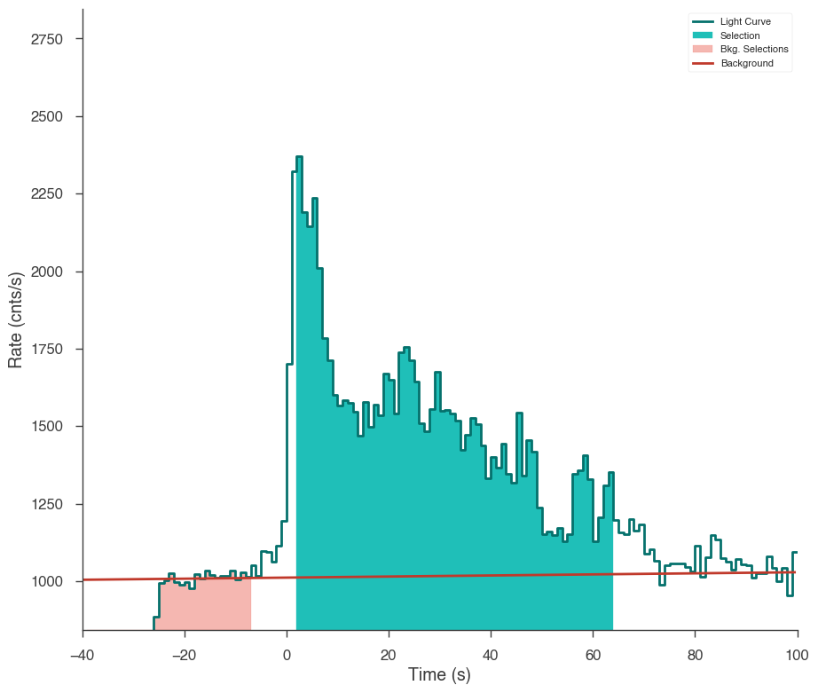
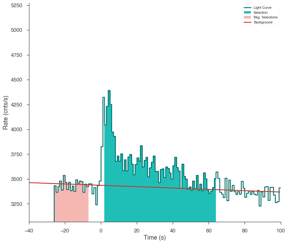
Let’s first examine the catalog fluence fit. Using the TimeSeriesBuilder, we can fit the background, set the source interval, and create a 3ML plugin for the analysis. We will loop through the detectors, set their appropriate channel selections, and ensure there are enough counts in each bin to make the PGStat profile likelihood valid.
First we use the CSPEC data to fit the background using the background selections. We use CSPEC because it has a longer duration for fitting the background.
The background is saved to an HDF5 file that stores the polynomial coefficients and selections which we can read in to the TTE file later.
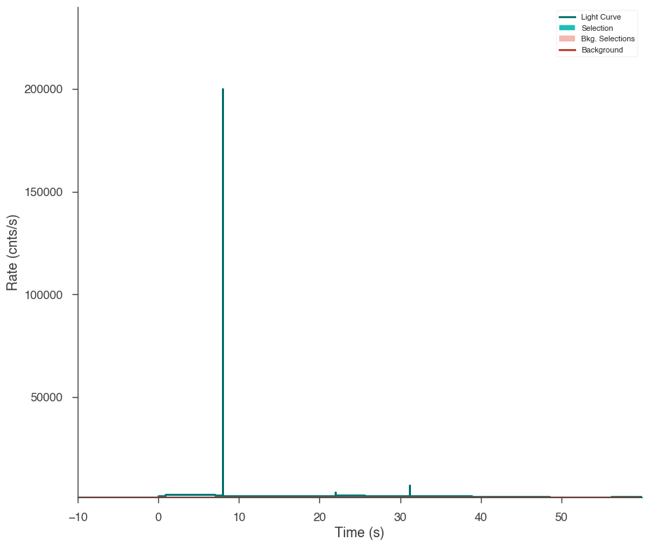
The light curve is plotted.
The source selection from the catalog is set and DispersionSpectrumLike plugin is created.
The plugin has the standard GBM channel selections for spectral analysis set.
[8]:
fluence_plugins = []
time_series = {}
for det in gbm_detectors:

    ts_cspec = TimeSeriesBuilder.from_gbm_cspec_or_ctime(
        det, cspec_or_ctime_file=dload[det]["cspec"], rsp_file=dload[det]["rsp"]
    )

    ts_cspec.set_background_interval(*background_interval.split(","))
    ts_cspec.save_background(f"{det}_bkg.h5", overwrite=True)

    ts_tte = TimeSeriesBuilder.from_gbm_tte(
        det,
        tte_file=dload[det]["tte"],
        rsp_file=dload[det]["rsp"],
        restore_background=f"{det}_bkg.h5",
    )

    time_series[det] = ts_tte

    ts_tte.set_active_time_interval(source_interval)

    ts_tte.view_lightcurve(-40, 100)

    fluence_plugin = ts_tte.to_spectrumlike()

    if det.startswith("b"):

        fluence_plugin.set_active_measurements("250-30000")

    else:

        fluence_plugin.set_active_measurements("9-900")

    fluence_plugin.rebin_on_background(1.0)

    fluence_plugins.append(fluence_plugin)
23:26:38 INFO Auto-determined polynomial order: 0 binned_spectrum_series.py:356
23:26:44 INFO None 0-order polynomial fit with the mle method time_series.py:426
INFO Saved fitted background to n3_bkg.h5 time_series.py:972
INFO Saved background to n3_bkg.h5 time_series_builder.py:430
INFO Successfully restored fit from n3_bkg.h5 time_series_builder.py:166
INFO Interval set to 1.28-64.257 for n3 time_series_builder.py:274
INFO Auto-probed noise models: SpectrumLike.py:486
INFO - observation: poisson SpectrumLike.py:487
INFO - background: gaussian SpectrumLike.py:488
INFO Range 9-900 translates to channels 5-124 SpectrumLike.py:1237
23:26:48 INFO Now using 120 bins SpectrumLike.py:1706
23:26:49 INFO Auto-determined polynomial order: 1 binned_spectrum_series.py:356
23:26:55 INFO None 1-order polynomial fit with the mle method time_series.py:426
INFO Saved fitted background to n4_bkg.h5 time_series.py:972
INFO Saved background to n4_bkg.h5 time_series_builder.py:430
INFO Successfully restored fit from n4_bkg.h5 time_series_builder.py:166
INFO Interval set to 1.28-64.257 for n4 time_series_builder.py:274
INFO Auto-probed noise models: SpectrumLike.py:486
INFO - observation: poisson SpectrumLike.py:487
INFO - background: gaussian SpectrumLike.py:488
INFO Range 9-900 translates to channels 5-123 SpectrumLike.py:1237
INFO Now using 119 bins SpectrumLike.py:1706
23:26:56 INFO Auto-determined polynomial order: 1 binned_spectrum_series.py:356
23:27:02 INFO None 1-order polynomial fit with the mle method time_series.py:426
INFO Saved fitted background to b0_bkg.h5 time_series.py:972
INFO Saved background to b0_bkg.h5 time_series_builder.py:430
INFO Successfully restored fit from b0_bkg.h5 time_series_builder.py:166
INFO Interval set to 1.28-64.257 for b0 time_series_builder.py:274
INFO Auto-probed noise models: SpectrumLike.py:486
INFO - observation: poisson SpectrumLike.py:487
INFO - background: gaussian SpectrumLike.py:488
INFO Range 250-30000 translates to channels 1-119 SpectrumLike.py:1237
INFO Now using 119 bins SpectrumLike.py:1706
Setting up the fit
Let’s see if we can reproduce the results from the catalog.
Set priors for the model
We will fit the spectrum using Bayesian analysis, so we must set priors on the model parameters.
[9]:
model.GRB080916009.spectrum.main.shape.alpha.prior = Truncated_gaussian(
    lower_bound=-1.5, upper_bound=1, mu=-1, sigma=0.5
)
model.GRB080916009.spectrum.main.shape.beta.prior = Truncated_gaussian(
    lower_bound=-5, upper_bound=-1.6, mu=-2.25, sigma=0.5
)
model.GRB080916009.spectrum.main.shape.break_energy.prior = Log_normal(mu=2, sigma=1)
model.GRB080916009.spectrum.main.shape.break_energy.bounds = (None, None)
model.GRB080916009.spectrum.main.shape.K.prior = Log_uniform_prior(
    lower_bound=1e-3, upper_bound=1e1
)
model.GRB080916009.spectrum.main.shape.break_scale.prior = Log_uniform_prior(
    lower_bound=1e-4, upper_bound=10
)
Clone the model and setup the Bayesian analysis class
Next, we clone the model we built from the catalog so that we can look at the results later and fit the cloned model. We pass this model and the DataList of the plugins to a BayesianAnalysis class and set the sampler to MultiNest.
[10]:
new_model = clone_model(model)

bayes = BayesianAnalysis(new_model, DataList(*fluence_plugins))

# share spectrum gives a linear speed up when
# spectrumlike plugins have the same RSP input energies
bayes.set_sampler("multinest", share_spectrum=True)
23:27:03 INFO sampler set to multinest bayesian_analysis.py:186
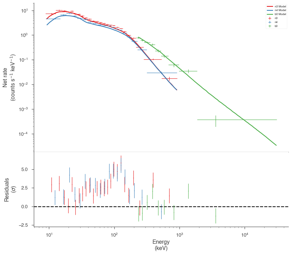
Examine at the catalog fitted model
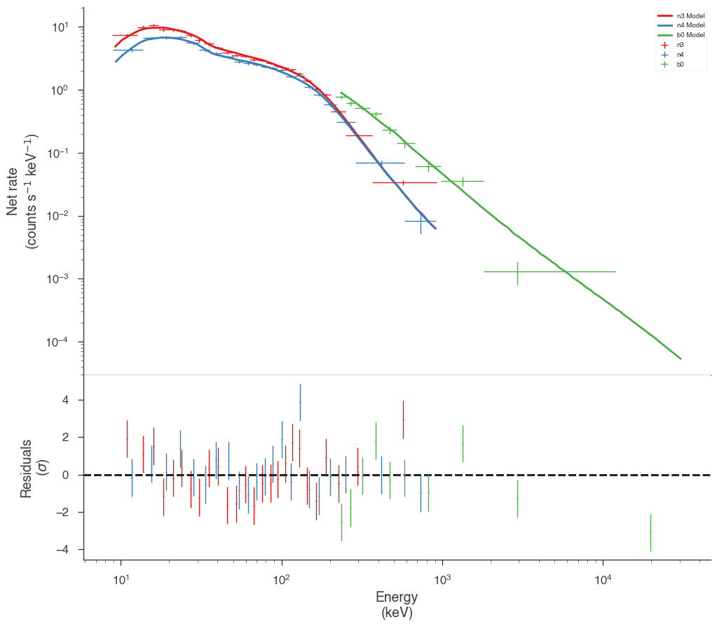
We can quickly examine how well the catalog fit matches the data. There appears to be a discrepancy between the data and the model! Let’s refit to see if we can fix it.
[11]:
fig = display_spectrum_model_counts(bayes, min_rate=20, step=False)
Run the sampler
We let MultiNest condition the model on the data
[12]:
bayes.sampler.setup(n_live_points=400)
bayes.sample()
 *****************************************************
 MultiNest v3.10
 Copyright Farhan Feroz & Mike Hobson
 Release Jul 2015

 no. of live points =  400
 dimensionality =    5
 *****************************************************
  analysing data from chains/fit-.txt ln(ev)=  -3102.4646875522662      +/-  0.23393269297960334
 Total Likelihood Evaluations:        21699
 Sampling finished. Exiting MultiNest
23:27:14 INFO fit restored to maximum of posterior sampler_base.py:168
INFO fit restored to maximum of posterior sampler_base.py:168
Maximum a posteriori probability (MAP) point:
| result | unit | |
|---|---|---|
| parameter | ||
| GRB080916009...K | (1.473 -0.023 +0.012) x 10^-2 | 1 / (keV s cm2) |
| GRB080916009...alpha | -1.078 -0.011 +0.025 | |
| GRB080916009...break_energy | (2.21 -0.17 +0.35) x 10^2 | keV |
| GRB080916009...break_scale | (2.2 -0.4 +1.3) x 10^-1 | |
| GRB080916009...beta | -2.08 -0.09 +0.07 |
Values of -log(posterior) at the minimum:
| -log(posterior) | |
|---|---|
| n3 | -1025.572013 |
| n4 | -1017.449908 |
| b0 | -1055.599640 |
| total | -3098.621562 |
Values of statistical measures:
| statistical measures | |
|---|---|
| AIC | 6207.413578 |
| BIC | 6226.645788 |
| DIC | 6178.655147 |
| PDIC | 3.675939 |
| log(Z) | -1347.383294 |
Now our model seems to match much better with the data!
[13]:
bayes.restore_median_fit()
fig = display_spectrum_model_counts(bayes, min_rate=20)
INFO fit restored to median of posterior sampler_base.py:157
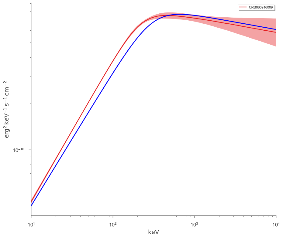
But how different are we from the catalog model? Let’s plot our fit along with the catalog model. Luckily, 3ML can handle all the units for is
[14]:
conversion = u.Unit("keV2/(cm2 s keV)").to("erg2/(cm2 s keV)")
energy_grid = np.logspace(1, 4, 100) * u.keV
vFv = (energy_grid**2 * model.get_point_source_fluxes(0, energy_grid)).to(
    "erg2/(cm2 s keV)"
)
[15]:
fig = plot_spectra(bayes.results, flux_unit="erg2/(cm2 s keV)")
ax = fig.get_axes()[0]
_ = ax.loglog(energy_grid, vFv, color="blue", label="catalog model")
Time Resolved Analysis
Now that we have examined fluence fit, we can move to performing a time-resolved analysis.
Selecting a temporal binning
We first get the brightest NaI detector and create time bins via the Bayesian blocks algorithm. We can use the fitted background to make sure that our intervals are chosen in an unbiased way.
[16]:
n3 = time_series["n3"]
[17]:
n3.create_time_bins(0, 60, method="bayesblocks", use_background=True, p0=0.2)
23:28:08 INFO Created 15 bins via bayesblocks time_series_builder.py:632
Sometimes, glitches in the GBM data cause spikes in the data that the Bayesian blocks algorithm detects as fast changes in the count rate. We will have to remove those intervals manually.
Note: In the future, 3ML will provide an automated method to remove these unwanted spikes.
[18]:
fig = n3.view_lightcurve(use_binner=True)
[19]:
bad_bins = []
for i, w in enumerate(n3.bins.widths):

    if w < 5e-2:
        bad_bins.append(i)


edges = [n3.bins.starts[0]]

for i, b in enumerate(n3.bins):

    if i not in bad_bins:
        edges.append(b.stop)

starts = edges[:-1]
stops = edges[1:]


n3.create_time_bins(starts, stops, method="custom")
23:28:09 INFO Created 12 bins via custom time_series_builder.py:632
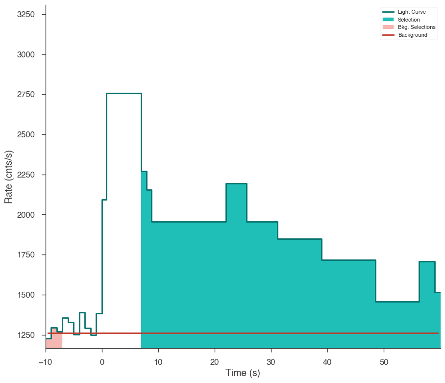
Now our light curve looks much more acceptable.
[20]:
fig = n3.view_lightcurve(use_binner=True)
The time series objects can read time bins from each other, so we will map these time bins onto the other detectors’ time series and create a list of time plugins for each detector and each time bin created above.
[21]:
time_resolved_plugins = {}

for k, v in time_series.items():
    v.read_bins(n3)
    time_resolved_plugins[k] = v.to_spectrumlike(from_bins=True)
INFO Created 12 bins via custom time_series_builder.py:632
INFO Interval set to 1.28-64.257 for n3 time_series_builder.py:274
INFO Created 12 bins via custom time_series_builder.py:632
INFO Interval set to 1.28-64.257 for n4 time_series_builder.py:274
INFO Created 12 bins via custom time_series_builder.py:632
23:28:10 INFO Interval set to 1.28-64.257 for b0 time_series_builder.py:274
Setting up the model
For the time-resolved analysis, we will fit the classic Band function to the data. We will set some principled priors.
[22]:
band = Band()
band.alpha.prior = Truncated_gaussian(lower_bound=-1.5, upper_bound=1, mu=-1, sigma=0.5)
band.beta.prior = Truncated_gaussian(lower_bound=-5, upper_bound=-1.6, mu=-2, sigma=0.5)
band.xp.prior = Log_normal(mu=2, sigma=1)
band.xp.bounds = (None, None)
band.K.prior = Log_uniform_prior(lower_bound=1e-10, upper_bound=1e3)
ps = PointSource("grb", 0, 0, spectral_shape=band)
band_model = Model(ps)
Perform the fits
One way to perform Bayesian spectral fits to all the intervals is to loop through each one. There can are many ways to do this, so find an analysis pattern that works for you.
[23]:
models = []
results = []
analysis = []
for interval in range(12):

    # clone the model above so that we have a separate model
    # for each fit

    this_model = clone_model(band_model)

    # for each detector set up the plugin
    # for this time interval

    this_data_list = []
    for k, v in time_resolved_plugins.items():

        pi = v[interval]

        if k.startswith("b"):
            pi.set_active_measurements("250-30000")
        else:
            pi.set_active_measurements("9-900")

        pi.rebin_on_background(1.0)

        this_data_list.append(pi)

    # create a data list

    dlist = DataList(*this_data_list)

    # set up the sampler and fit

    bayes = BayesianAnalysis(this_model, dlist)

    # get some speed with share spectrum
    bayes.set_sampler("multinest", share_spectrum=True)
    bayes.sampler.setup(n_live_points=500)
    bayes.sample()

    # at this stage we coudl also
    # save the analysis result to
    # disk but we will simply hold
    # onto them in memory

    analysis.append(bayes)
INFO Range 9-900 translates to channels 5-124 SpectrumLike.py:1237
INFO Now using 120 bins SpectrumLike.py:1706
INFO Range 9-900 translates to channels 5-123 SpectrumLike.py:1237
INFO Now using 119 bins SpectrumLike.py:1706
INFO Range 250-30000 translates to channels 1-119 SpectrumLike.py:1237
INFO Now using 107 bins SpectrumLike.py:1706
INFO sampler set to multinest bayesian_analysis.py:186
 *****************************************************
 MultiNest v3.10
 Copyright Farhan Feroz & Mike Hobson
 Release Jul 2015

 no. of live points =  500
 dimensionality =    4
 *****************************************************
  analysing data from chains/fit-.txt
 ln(ev)=  -788.33008951143381      +/-  0.17629316121659205
 Total Likelihood Evaluations:        16169
 Sampling finished. Exiting MultiNest
23:28:19 INFO fit restored to maximum of posterior sampler_base.py:168
INFO fit restored to maximum of posterior sampler_base.py:168
Maximum a posteriori probability (MAP) point:
| result | unit | |
|---|---|---|
| parameter | ||
| grb.spectrum.main.Band.K | (3.5 -0.5 +0.7) x 10^-2 | 1 / (keV s cm2) |
| grb.spectrum.main.Band.alpha | (-5.8 -1.0 +1.5) x 10^-1 | |
| grb.spectrum.main.Band.xp | (3.2 -0.5 +0.8) x 10^2 | keV |
| grb.spectrum.main.Band.beta | -2.05 -0.4 +0.07 |
Values of -log(posterior) at the minimum:
| -log(posterior) | |
|---|---|
| n3_interval0 | -250.238374 |
| n4_interval0 | -268.017730 |
| b0_interval0 | -285.697807 |
| total | -803.953910 |
Values of statistical measures:
| statistical measures | |
|---|---|
| AIC | 1616.021134 |
| BIC | 1631.429952 |
| DIC | 1570.523423 |
| PDIC | 2.345517 |
| log(Z) | -342.367408 |
INFO Range 9-900 translates to channels 5-124 SpectrumLike.py:1237
INFO Now using 120 bins SpectrumLike.py:1706
INFO Range 9-900 translates to channels 5-123 SpectrumLike.py:1237
INFO Now using 119 bins SpectrumLike.py:1706
INFO Range 250-30000 translates to channels 1-119 SpectrumLike.py:1237
INFO Now using 119 bins SpectrumLike.py:1706
INFO sampler set to multinest bayesian_analysis.py:186
 *****************************************************
 MultiNest v3.10
 Copyright Farhan Feroz & Mike Hobson
 Release Jul 2015

 no. of live points =  500
 dimensionality =    4
 *****************************************************
  analysing data from chains/fit-.txt ln(ev)=  -1976.1204375554225      +/-  0.23942524602187540
 Total Likelihood Evaluations:        25296
 Sampling finished. Exiting MultiNest
23:28:36 INFO fit restored to maximum of posterior sampler_base.py:168
INFO fit restored to maximum of posterior sampler_base.py:168
Maximum a posteriori probability (MAP) point:
| result | unit | |
|---|---|---|
| parameter | ||
| grb.spectrum.main.Band.K | (3.97 -0.08 +0.04) x 10^-2 | 1 / (keV s cm2) |
| grb.spectrum.main.Band.alpha | (-9.78 -0.17 +0.10) x 10^-1 | |
| grb.spectrum.main.Band.xp | (7.4 -0.5 +0.7) x 10^2 | keV |
| grb.spectrum.main.Band.beta | -2.420 -0.05 +0.009 |
Values of -log(posterior) at the minimum:
| -log(posterior) | |
|---|---|
| n3_interval1 | -660.899630 |
| n4_interval1 | -656.928102 |
| b0_interval1 | -674.078870 |
| total | -1991.906601 |
Values of statistical measures:
| statistical measures | |
|---|---|
| AIC | 3991.926517 |
| BIC | 4007.335335 |
| DIC | 3926.927323 |
| PDIC | 1.486764 |
| log(Z) | -858.218202 |
INFO Range 9-900 translates to channels 5-124 SpectrumLike.py:1237
INFO Now using 120 bins SpectrumLike.py:1706
INFO Range 9-900 translates to channels 5-123 SpectrumLike.py:1237
INFO Now using 119 bins SpectrumLike.py:1706
INFO Range 250-30000 translates to channels 1-119 SpectrumLike.py:1237
INFO Now using 115 bins SpectrumLike.py:1706
INFO sampler set to multinest bayesian_analysis.py:186
 *****************************************************
 MultiNest v3.10
 Copyright Farhan Feroz & Mike Hobson
 Release Jul 2015

 no. of live points =  500
 dimensionality =    4
 *****************************************************
  analysing data from chains/fit-.txt
 ln(ev)=  -908.00105881226455      +/-  0.19837698079850238
 Total Likelihood Evaluations:        19148
 Sampling finished. Exiting MultiNest
23:28:48 INFO fit restored to maximum of posterior sampler_base.py:168
INFO fit restored to maximum of posterior sampler_base.py:168
Maximum a posteriori probability (MAP) point:
| result | unit | |
|---|---|---|
| parameter | ||
| grb.spectrum.main.Band.K | (2.59 -0.08 +0.30) x 10^-2 | 1 / (keV s cm2) |
| grb.spectrum.main.Band.alpha | -1.02 -0.04 +0.07 | |
| grb.spectrum.main.Band.xp | (5.6 -1.2 +1.0) x 10^2 | keV |
| grb.spectrum.main.Band.beta | -1.927 -0.19 -0.016 |
Values of -log(posterior) at the minimum:
| -log(posterior) | |
|---|---|
| n3_interval2 | -288.719335 |
| n4_interval2 | -312.664892 |
| b0_interval2 | -324.252491 |
| total | -925.636718 |
Values of statistical measures:
| statistical measures | |
|---|---|
| AIC | 1859.386750 |
| BIC | 1874.795568 |
| DIC | 1804.063173 |
| PDIC | 1.744937 |
| log(Z) | -394.339849 |
INFO Range 9-900 translates to channels 5-124 SpectrumLike.py:1237
INFO Now using 120 bins SpectrumLike.py:1706
INFO Range 9-900 translates to channels 5-123 SpectrumLike.py:1237
INFO Now using 119 bins SpectrumLike.py:1706
INFO Range 250-30000 translates to channels 1-119 SpectrumLike.py:1237
INFO Now using 109 bins SpectrumLike.py:1706
INFO sampler set to multinest bayesian_analysis.py:186
 *****************************************************
 MultiNest v3.10
 Copyright Farhan Feroz & Mike Hobson
 Release Jul 2015

 no. of live points =  500
 dimensionality =    4
 *****************************************************
  analysing data from chains/fit-.txt
 ln(ev)=  -788.72961727063330      +/-  0.18023507827422039
 Total Likelihood Evaluations:        16881
 Sampling finished. Exiting MultiNest
23:28:57 INFO fit restored to maximum of posterior sampler_base.py:168
INFO fit restored to maximum of posterior sampler_base.py:168
Maximum a posteriori probability (MAP) point:
| result | unit | |
|---|---|---|
| parameter | ||
| grb.spectrum.main.Band.K | (2.89 -0.23 +0.4) x 10^-2 | 1 / (keV s cm2) |
| grb.spectrum.main.Band.alpha | (-9.2 -0.6 +0.8) x 10^-1 | |
| grb.spectrum.main.Band.xp | (3.4 +/- 0.6) x 10^2 | keV |
| grb.spectrum.main.Band.beta | -2.28 -0.27 +0.12 |
Values of -log(posterior) at the minimum:
| -log(posterior) | |
|---|---|
| n3_interval3 | -242.555978 |
| n4_interval3 | -262.676390 |
| b0_interval3 | -298.405355 |
| total | -803.637723 |
Values of statistical measures:
| statistical measures | |
|---|---|
| AIC | 1615.388760 |
| BIC | 1630.797577 |
| DIC | 1569.127414 |
| PDIC | 2.362850 |
| log(Z) | -342.540920 |
INFO Range 9-900 translates to channels 5-124 SpectrumLike.py:1237
INFO Now using 120 bins SpectrumLike.py:1706
INFO Range 9-900 translates to channels 5-123 SpectrumLike.py:1237
INFO Now using 119 bins SpectrumLike.py:1706
INFO Range 250-30000 translates to channels 1-119 SpectrumLike.py:1237
INFO Now using 119 bins SpectrumLike.py:1706
INFO sampler set to multinest bayesian_analysis.py:186
 *****************************************************
 MultiNest v3.10
 Copyright Farhan Feroz & Mike Hobson
 Release Jul 2015

 no. of live points =  500
 dimensionality =    4
 *****************************************************
  analysing data from chains/fit-.txt ln(ev)=  -2270.1707479940942      +/-  0.19561584225580966
 Total Likelihood Evaluations:        22689
 Sampling finished. Exiting MultiNest
23:29:08 INFO fit restored to maximum of posterior sampler_base.py:168
INFO fit restored to maximum of posterior sampler_base.py:168
Maximum a posteriori probability (MAP) point:
| result | unit | |
|---|---|---|
| parameter | ||
| grb.spectrum.main.Band.K | (2.02 -0.12 +0.06) x 10^-2 | 1 / (keV s cm2) |
| grb.spectrum.main.Band.alpha | (-9.9 +/- 0.4) x 10^-1 | |
| grb.spectrum.main.Band.xp | (4.02 -0.10 +0.9) x 10^2 | keV |
| grb.spectrum.main.Band.beta | -1.948 -0.16 +0.013 |
Values of -log(posterior) at the minimum:
| -log(posterior) | |
|---|---|
| n3_interval4 | -756.914439 |
| n4_interval4 | -747.169689 |
| b0_interval4 | -778.471687 |
| total | -2282.555816 |
Values of statistical measures:
| statistical measures | |
|---|---|
| AIC | 4573.224946 |
| BIC | 4588.633764 |
| DIC | 4528.516278 |
| PDIC | 3.552112 |
| log(Z) | -985.922629 |
INFO Range 9-900 translates to channels 5-124 SpectrumLike.py:1237
INFO Now using 120 bins SpectrumLike.py:1706
INFO Range 9-900 translates to channels 5-123 SpectrumLike.py:1237
INFO Now using 119 bins SpectrumLike.py:1706
INFO Range 250-30000 translates to channels 1-119 SpectrumLike.py:1237
INFO Now using 119 bins SpectrumLike.py:1706
INFO sampler set to multinest bayesian_analysis.py:186
 *****************************************************
 MultiNest v3.10
 Copyright Farhan Feroz & Mike Hobson
 Release Jul 2015

 no. of live points =  500
 dimensionality =    4
 *****************************************************
  analysing data from chains/fit-.txt
 ln(ev)=  -1588.7151568878458      +/-  0.22559505663194443
 Total Likelihood Evaluations:        19929
 Sampling finished. Exiting MultiNest
23:29:20 INFO fit restored to maximum of posterior sampler_base.py:168
INFO fit restored to maximum of posterior sampler_base.py:168
Maximum a posteriori probability (MAP) point:
| result | unit | |
|---|---|---|
| parameter | ||
| grb.spectrum.main.Band.K | (2.727 +0.029 +0.17) x 10^-2 | 1 / (keV s cm2) |
| grb.spectrum.main.Band.alpha | (-9.98 -0.08 +0.09) x 10^-1 | |
| grb.spectrum.main.Band.xp | (4.34 -0.7 -0.15) x 10^2 | keV |
| grb.spectrum.main.Band.beta | -1.923 -0.020 +0.007 |
Values of -log(posterior) at the minimum:
| -log(posterior) | |
|---|---|
| n3_interval5 | -523.057487 |
| n4_interval5 | -532.592650 |
| b0_interval5 | -538.902171 |
| total | -1594.552308 |
Values of statistical measures:
| statistical measures | |
|---|---|
| AIC | 3197.217931 |
| BIC | 3212.626748 |
| DIC | 3150.506033 |
| PDIC | 1.377681 |
| log(Z) | -689.970226 |
INFO Range 9-900 translates to channels 5-124 SpectrumLike.py:1237
INFO Now using 120 bins SpectrumLike.py:1706
INFO Range 9-900 translates to channels 5-123 SpectrumLike.py:1237
INFO Now using 119 bins SpectrumLike.py:1706
INFO Range 250-30000 translates to channels 1-119 SpectrumLike.py:1237
INFO Now using 119 bins SpectrumLike.py:1706
INFO sampler set to multinest bayesian_analysis.py:186
 *****************************************************
 MultiNest v3.10
 Copyright Farhan Feroz & Mike Hobson
 Release Jul 2015

 no. of live points =  500
 dimensionality =    4
 *****************************************************
  analysing data from chains/fit-.txt ln(ev)=  -1756.6034716144832      +/-  0.19530310687040472
 Total Likelihood Evaluations:        19484
 Sampling finished. Exiting MultiNest
23:29:30 INFO fit restored to maximum of posterior sampler_base.py:168
INFO fit restored to maximum of posterior sampler_base.py:168
Maximum a posteriori probability (MAP) point:
| result | unit | |
|---|---|---|
| parameter | ||
| grb.spectrum.main.Band.K | (1.93 +0.05 +0.26) x 10^-2 | 1 / (keV s cm2) |
| grb.spectrum.main.Band.alpha | -1.0212 +0.0033 +0.09 | |
| grb.spectrum.main.Band.xp | (4.60 -1.0 -0.28) x 10^2 | keV |
| grb.spectrum.main.Band.beta | -2.36 -0.12 +0.21 |
Values of -log(posterior) at the minimum:
| -log(posterior) | |
|---|---|
| n3_interval6 | -584.327319 |
| n4_interval6 | -576.984599 |
| b0_interval6 | -609.663253 |
| total | -1770.975171 |
Values of statistical measures:
| statistical measures | |
|---|---|
| AIC | 3550.063656 |
| BIC | 3565.472473 |
| DIC | 3500.082552 |
| PDIC | 2.533090 |
| log(Z) | -762.883195 |
INFO Range 9-900 translates to channels 5-124 SpectrumLike.py:1237
INFO Now using 120 bins SpectrumLike.py:1706
INFO Range 9-900 translates to channels 5-123 SpectrumLike.py:1237
INFO Now using 119 bins SpectrumLike.py:1706
INFO Range 250-30000 translates to channels 1-119 SpectrumLike.py:1237
INFO Now using 119 bins SpectrumLike.py:1706
INFO sampler set to multinest bayesian_analysis.py:186
 *****************************************************
 MultiNest v3.10
 Copyright Farhan Feroz & Mike Hobson
 Release Jul 2015

 no. of live points =  500
 dimensionality =    4
 *****************************************************
  analysing data from chains/fit-.txt
 ln(ev)=  -1938.8598068271624      +/-  0.18930080622273393
 Total Likelihood Evaluations:        22284
 Sampling finished. Exiting MultiNest
23:29:40 INFO fit restored to maximum of posterior sampler_base.py:168
INFO fit restored to maximum of posterior sampler_base.py:168
Maximum a posteriori probability (MAP) point:
| result | unit | |
|---|---|---|
| parameter | ||
| grb.spectrum.main.Band.K | (1.66 -0.11 +0.09) x 10^-2 | 1 / (keV s cm2) |
| grb.spectrum.main.Band.alpha | -1.05 -0.05 +0.04 | |
| grb.spectrum.main.Band.xp | (4.3 -0.4 +0.9) x 10^2 | keV |
| grb.spectrum.main.Band.beta | -2.25 -0.5 +0.11 |
Values of -log(posterior) at the minimum:
| -log(posterior) | |
|---|---|
| n3_interval7 | -640.797058 |
| n4_interval7 | -650.463422 |
| b0_interval7 | -662.335721 |
| total | -1953.596201 |
Values of statistical measures:
| statistical measures | |
|---|---|
| AIC | 3915.305716 |
| BIC | 3930.714533 |
| DIC | 3869.256959 |
| PDIC | 3.504752 |
| log(Z) | -842.036115 |
INFO Range 9-900 translates to channels 5-124 SpectrumLike.py:1237
INFO Now using 120 bins SpectrumLike.py:1706
INFO Range 9-900 translates to channels 5-123 SpectrumLike.py:1237
INFO Now using 119 bins SpectrumLike.py:1706
INFO Range 250-30000 translates to channels 1-119 SpectrumLike.py:1237
INFO Now using 119 bins SpectrumLike.py:1706
INFO sampler set to multinest bayesian_analysis.py:186
 *****************************************************
 MultiNest v3.10
 Copyright Farhan Feroz & Mike Hobson
 Release Jul 2015

 no. of live points =  500
 dimensionality =    4
 *****************************************************
  analysing data from chains/fit-.txt
 ln(ev)=  -2053.9234829574402      +/-  0.18765611114223760
 Total Likelihood Evaluations:        18609
 Sampling finished. Exiting MultiNest
23:29:49 INFO fit restored to maximum of posterior sampler_base.py:168
INFO fit restored to maximum of posterior sampler_base.py:168
Maximum a posteriori probability (MAP) point:
| result | unit | |
|---|---|---|
| parameter | ||
| grb.spectrum.main.Band.K | (1.54 -0.14 +0.12) x 10^-2 | 1 / (keV s cm2) |
| grb.spectrum.main.Band.alpha | (-8.4 -0.7 +0.6) x 10^-1 | |
| grb.spectrum.main.Band.xp | (3.7 -0.4 +0.7) x 10^2 | keV |
| grb.spectrum.main.Band.beta | -2.23 -0.5 +0.05 |
Values of -log(posterior) at the minimum:
| -log(posterior) | |
|---|---|
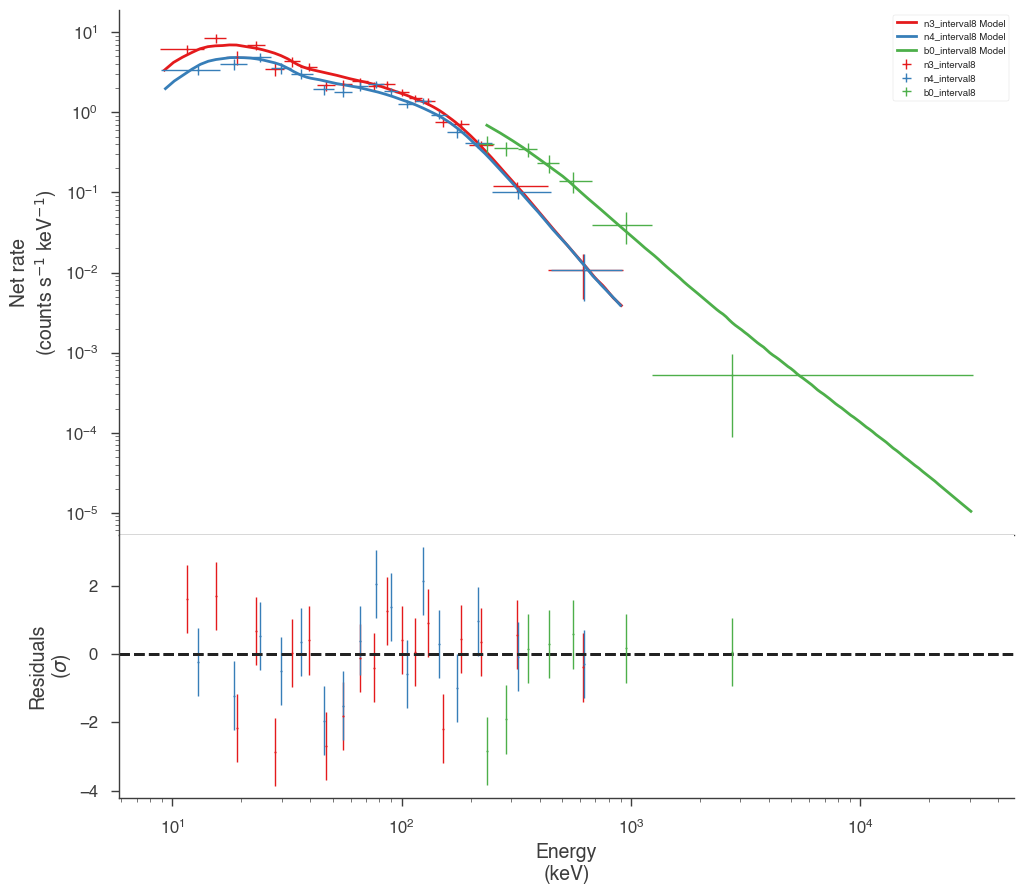
| n3_interval8 | -698.338333 |
| n4_interval8 | -665.939622 |
| b0_interval8 | -702.333851 |
| total | -2066.611806 |
Values of statistical measures:
| statistical measures | |
|---|---|
| AIC | 4141.336926 |
| BIC | 4156.745744 |
| DIC | 4098.200969 |
| PDIC | 3.288385 |
| log(Z) | -892.007635 |
INFO Range 9-900 translates to channels 5-124 SpectrumLike.py:1237
INFO Now using 120 bins SpectrumLike.py:1706
INFO Range 9-900 translates to channels 5-123 SpectrumLike.py:1237
INFO Now using 119 bins SpectrumLike.py:1706
INFO Range 250-30000 translates to channels 1-119 SpectrumLike.py:1237
INFO Now using 119 bins SpectrumLike.py:1706
INFO sampler set to multinest bayesian_analysis.py:186
 *****************************************************
 MultiNest v3.10
 Copyright Farhan Feroz & Mike Hobson
 Release Jul 2015

 no. of live points =  500
 dimensionality =    4
 *****************************************************
  analysing data from chains/fit-.txt ln(ev)=  -1878.5225350690589      +/-  0.14445595743358311
 Total Likelihood Evaluations:        12984
 Sampling finished. Exiting MultiNest
23:29:55 INFO fit restored to maximum of posterior sampler_base.py:168
INFO fit restored to maximum of posterior sampler_base.py:168
Maximum a posteriori probability (MAP) point:
| result | unit | |
|---|---|---|
| parameter | ||
| grb.spectrum.main.Band.K | (1.04 -0.31 +0.9) x 10^-2 | 1 / (keV s cm2) |
| grb.spectrum.main.Band.alpha | (-8.9 -1.8 +3.0) x 10^-1 | |
| grb.spectrum.main.Band.xp | (1.2 -0.4 +0.5) x 10^2 | keV |
| grb.spectrum.main.Band.beta | -1.92 -0.31 +0.18 |
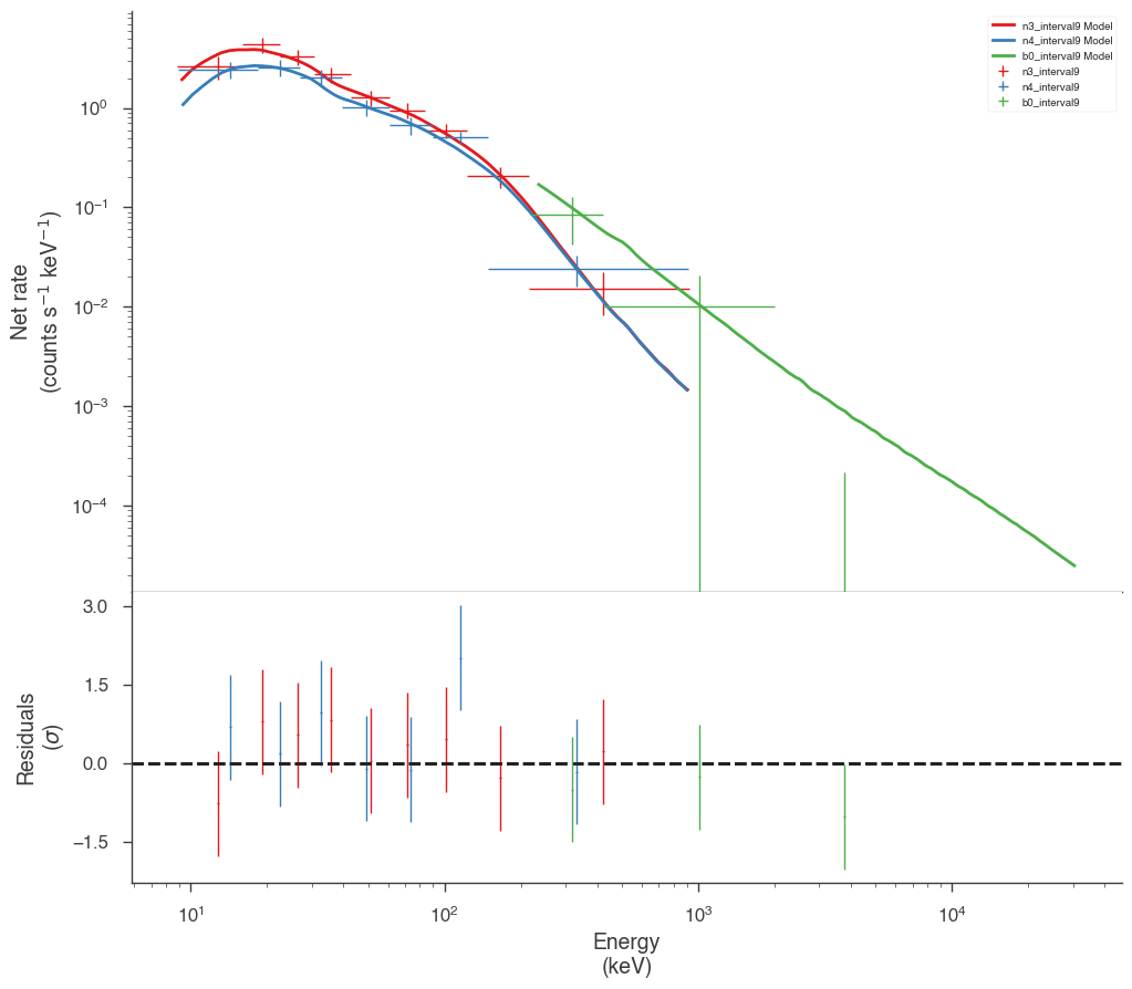
Values of -log(posterior) at the minimum:
| -log(posterior) | |
|---|---|
| n3_interval9 | -617.261226 |
| n4_interval9 | -616.395321 |
| b0_interval9 | -648.403457 |
| total | -1882.060005 |
Values of statistical measures:
| statistical measures | |
|---|---|
| AIC | 3772.233324 |
| BIC | 3787.642141 |
| DIC | 3712.493052 |
| PDIC | -34.670419 |
| log(Z) | -815.831971 |
INFO Range 9-900 translates to channels 5-124 SpectrumLike.py:1237
INFO Now using 120 bins SpectrumLike.py:1706
INFO Range 9-900 translates to channels 5-123 SpectrumLike.py:1237
INFO Now using 119 bins SpectrumLike.py:1706
INFO Range 250-30000 translates to channels 1-119 SpectrumLike.py:1237
INFO Now using 119 bins SpectrumLike.py:1706
INFO sampler set to multinest bayesian_analysis.py:186
 *****************************************************
 MultiNest v3.10
 Copyright Farhan Feroz & Mike Hobson
 Release Jul 2015

 no. of live points =  500
 dimensionality =    4
 *****************************************************
  analysing data from chains/fit-.txt ln(ev)=  -1323.3166676849601      +/-  0.17305437828887349
 Total Likelihood Evaluations:        15238
 Sampling finished. Exiting MultiNest
23:30:03 INFO fit restored to maximum of posterior sampler_base.py:168
INFO fit restored to maximum of posterior sampler_base.py:168
Maximum a posteriori probability (MAP) point:
| result | unit | |
|---|---|---|
| parameter | ||
| grb.spectrum.main.Band.K | (2.11 -0.13 +0.6) x 10^-2 | 1 / (keV s cm2) |
| grb.spectrum.main.Band.alpha | (-7.3 -0.4 +1.6) x 10^-1 | |
| grb.spectrum.main.Band.xp | (2.09 -0.4 +0.23) x 10^2 | keV |
| grb.spectrum.main.Band.beta | -1.92 -0.25 +0.04 |
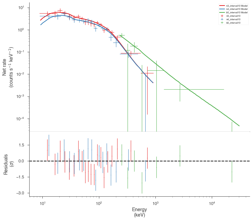
Values of -log(posterior) at the minimum:
| -log(posterior) | |
|---|---|
| n3_interval10 | -437.752009 |
| n4_interval10 | -432.913690 |
| b0_interval10 | -460.777976 |
| total | -1331.443675 |
Values of statistical measures:
| statistical measures | |
|---|---|
| AIC | 2671.000664 |
| BIC | 2686.409482 |
| DIC | 2632.673036 |
| PDIC | -0.427101 |
| log(Z) | -574.709127 |
INFO Range 9-900 translates to channels 5-124 SpectrumLike.py:1237
INFO Now using 120 bins SpectrumLike.py:1706
INFO Range 9-900 translates to channels 5-123 SpectrumLike.py:1237
INFO Now using 119 bins SpectrumLike.py:1706
INFO Range 250-30000 translates to channels 1-119 SpectrumLike.py:1237
INFO Now using 119 bins SpectrumLike.py:1706
INFO sampler set to multinest bayesian_analysis.py:186
 *****************************************************
 MultiNest v3.10
 Copyright Farhan Feroz & Mike Hobson
 Release Jul 2015

 no. of live points =  500
 dimensionality =    4
 *****************************************************
  analysing data from chains/fit-.txt ln(ev)=  -812.46443518169860      +/-  0.15106828584241486
 Total Likelihood Evaluations:        11941
 Sampling finished. Exiting MultiNest
23:30:09 INFO fit restored to maximum of posterior sampler_base.py:168
INFO fit restored to maximum of posterior sampler_base.py:168
Maximum a posteriori probability (MAP) point:
| result | unit | |
|---|---|---|
| parameter | ||
| grb.spectrum.main.Band.K | (3.1 -1.2 +0.9) x 10^-2 | 1 / (keV s cm2) |
| grb.spectrum.main.Band.alpha | (-4.5 -2.9 +1.9) x 10^-1 | |
| grb.spectrum.main.Band.xp | (1.22 -0.12 +0.4) x 10^2 | keV |
| grb.spectrum.main.Band.beta | -2.074 -0.6 -0.012 |
Values of -log(posterior) at the minimum:
| -log(posterior) | |
|---|---|
| n3_interval11 | -272.564103 |
| n4_interval11 | -255.659380 |
| b0_interval11 | -292.325537 |
| total | -820.549020 |
Values of statistical measures:
| statistical measures | |
|---|---|
| AIC | 1649.211354 |
| BIC | 1664.620171 |
| DIC | 1618.880848 |
| PDIC | 1.594778 |
| log(Z) | -352.848821 |
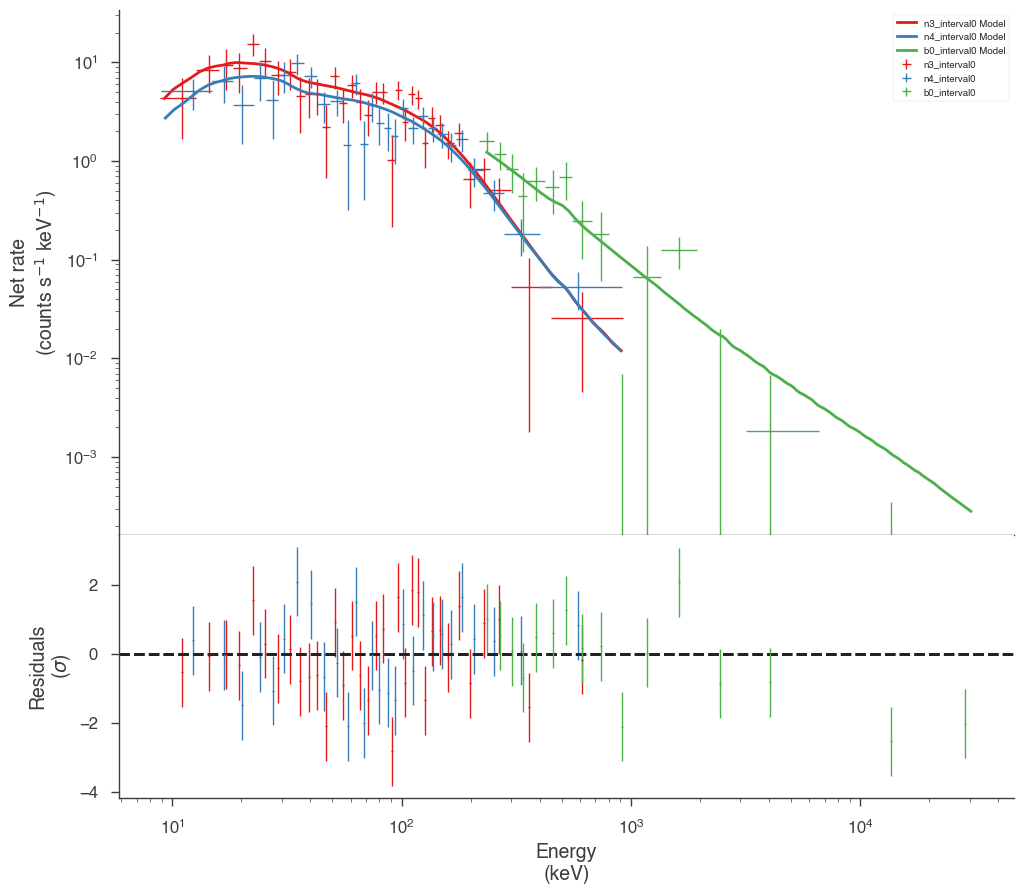
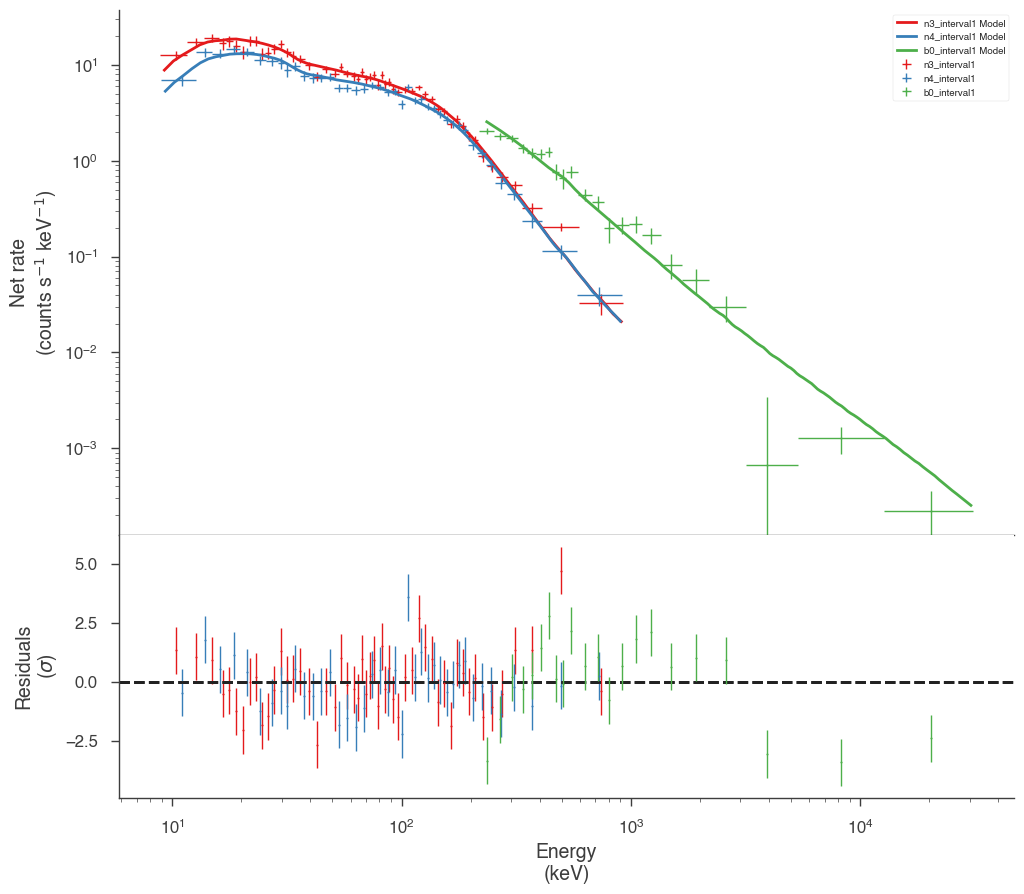
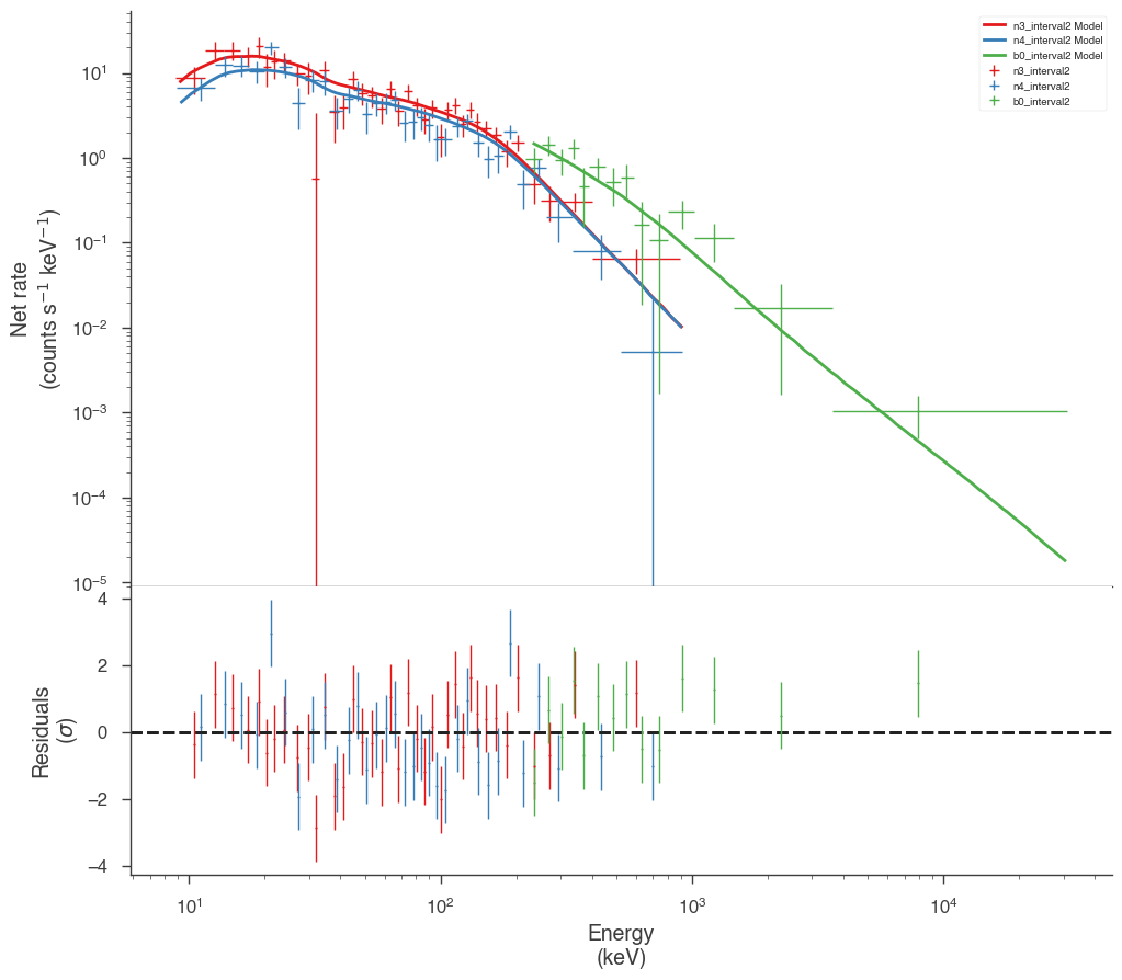
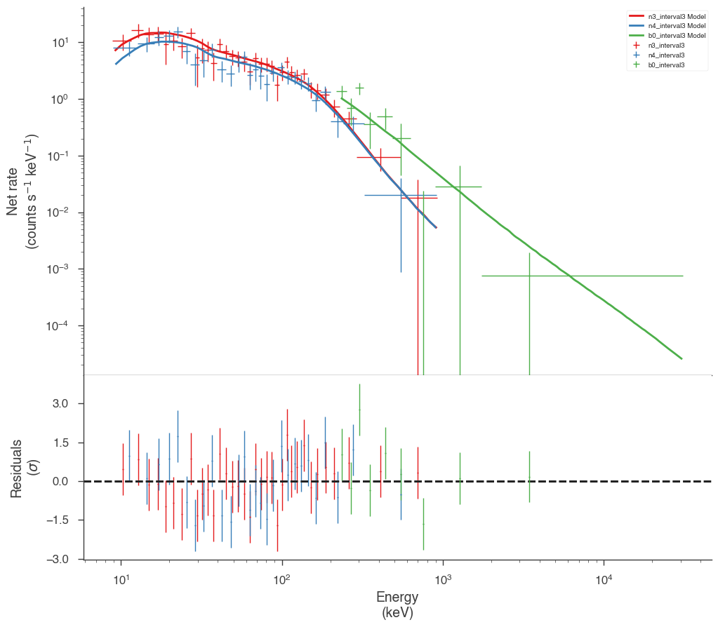
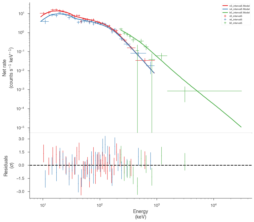
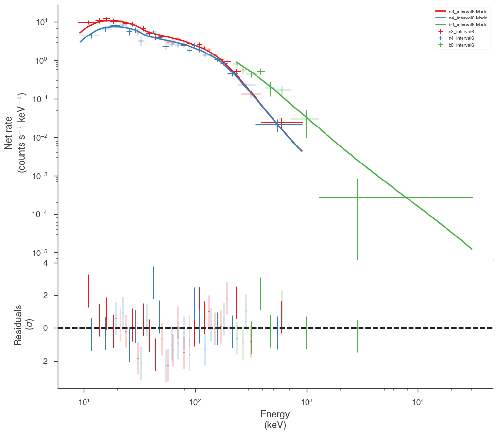
Examine the fits
Now we can look at the fits in count space to make sure they are ok.
[24]:
for a in analysis:
    a.restore_median_fit()
    _ = display_spectrum_model_counts(a, min_rate=[20, 20, 20], step=False)
INFO fit restored to median of posterior sampler_base.py:157
23:30:10 INFO fit restored to median of posterior sampler_base.py:157
INFO fit restored to median of posterior sampler_base.py:157
INFO fit restored to median of posterior sampler_base.py:157
23:30:11 INFO fit restored to median of posterior sampler_base.py:157
INFO fit restored to median of posterior sampler_base.py:157
23:30:12 INFO fit restored to median of posterior sampler_base.py:157
INFO fit restored to median of posterior sampler_base.py:157
INFO fit restored to median of posterior sampler_base.py:157
23:30:13 INFO fit restored to median of posterior sampler_base.py:157
INFO fit restored to median of posterior sampler_base.py:157
INFO fit restored to median of posterior sampler_base.py:157
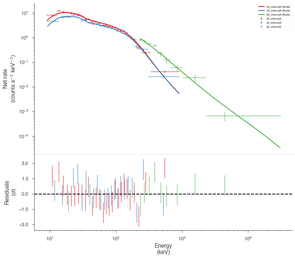
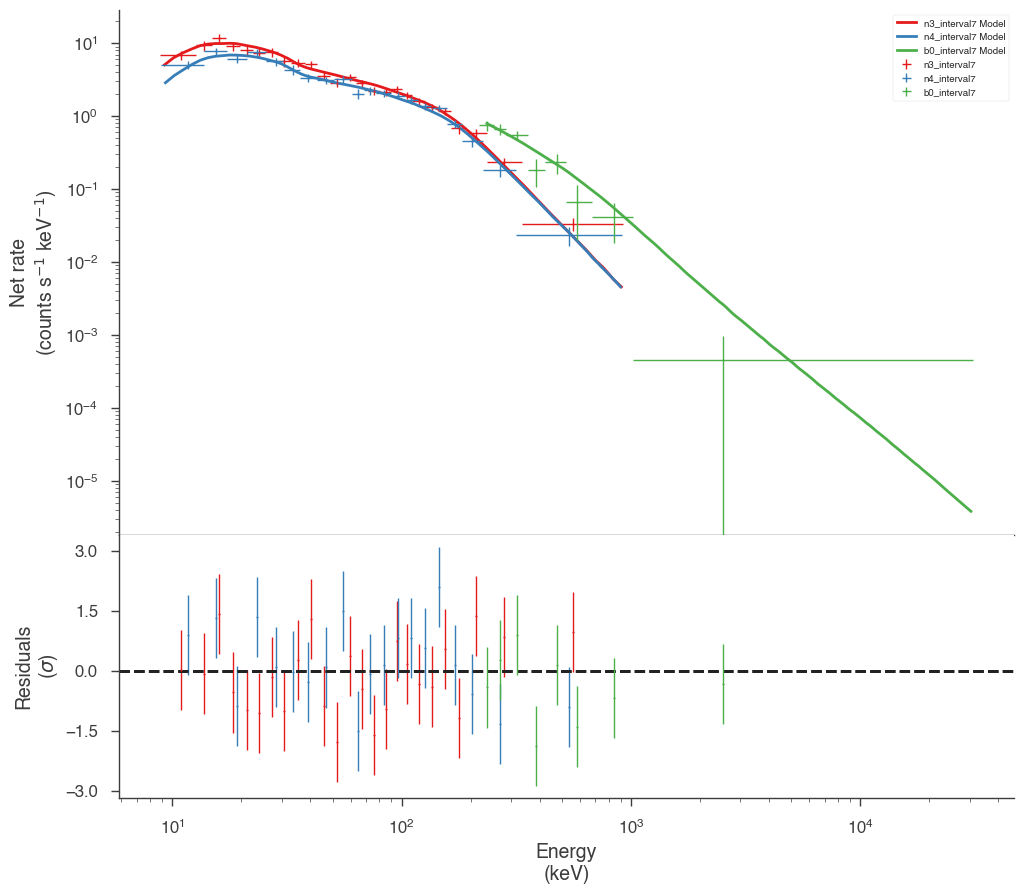
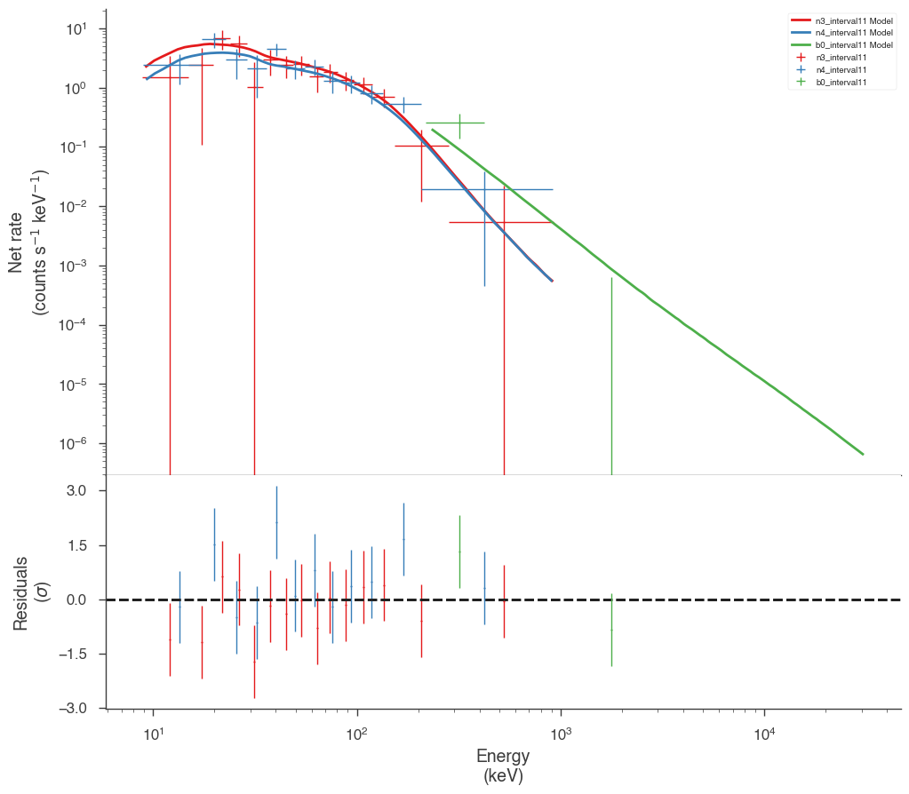
Finally, we can plot the models together to see how the spectra evolve with time.
[25]:
fig = plot_spectra(
    *[a.results for a in analysis[::1]],
    flux_unit="erg2/(cm2 s keV)",
    fit_cmap="viridis",
    contour_cmap="viridis",
    contour_style_kwargs=dict(alpha=0.1),
)
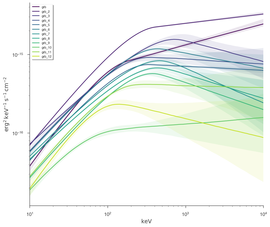
This example can serve as a template for performing analysis on GBM data. However, as 3ML provides an abstract interface and modular building blocks, similar analysis pipelines can be built for any time series data.