Joint fitting XRT and GBM data with XSPEC models

Goals

3ML is designed to properly joint fit data from different instruments with thier instrument dependent likelihoods. We demostrate this with joint fitting data from GBM and XRT while simultaneously showing hwo to use the XSPEC models form astromodels

Setup

You must have you HEASARC initiated so that astromodels can find the XSPEC libraries.

[1]:

import warnings

warnings.simplefilter("ignore")
import numpy as np

np.seterr(all="ignore")

[1]:

{'divide': 'warn', 'over': 'warn', 'under': 'ignore', 'invalid': 'warn'}

[2]:

%%capture
import matplotlib.pyplot as plt
from pathlib import Path
from threeML import *
from threeML.io.package_data import get_path_of_data_file

# we will need XPSEC models for extinction
from astromodels.xspec import *
from astromodels.xspec.xspec_settings import *

[3]:

from jupyterthemes import jtplot

%matplotlib inline
jtplot.style(context="talk", fscale=1, ticks=True, grid=False)
set_threeML_style()
silence_warnings()

Load XRT data

Make a likelihood for the XRT including all the appropriate files

[4]:

trigger = "GRB110731A"
dec = -28.546
ra = 280.52

p = Path("datasets/xrt")

xrt = OGIPLike(
    "XRT",
    observation=get_path_of_data_file(p / "xrt_src.pha"),
    background=get_path_of_data_file(p / "xrt_bkg.pha"),
    response=get_path_of_data_file(p / "xrt.rmf"),
    arf_file=get_path_of_data_file(p / "xrt.arf"),
)


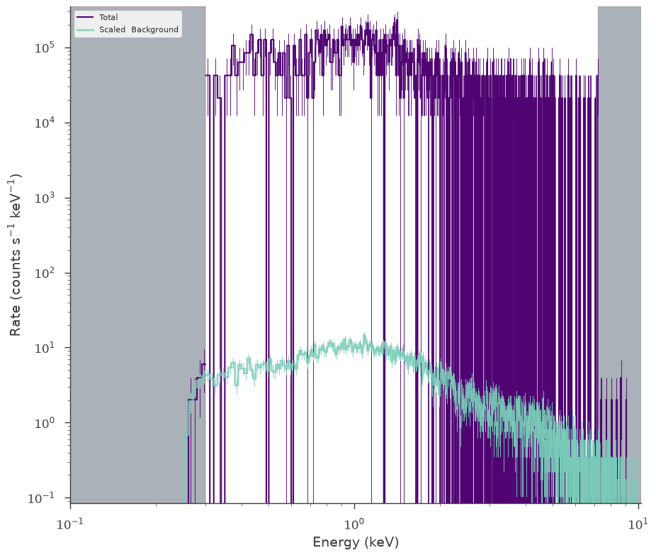
fig = xrt.view_count_spectrum()
ax = fig.get_axes()[0]
_ = ax.set_xlim(1e-1)

Found TSTOP and TELAPSE. This file is invalid. Using TSTOP.
Found TSTOP and TELAPSE. This file is invalid. Using TSTOP.

../_images/notebooks_joint_fitting_xrt_and_gbm_xspec_models_5_1.png

[5]:

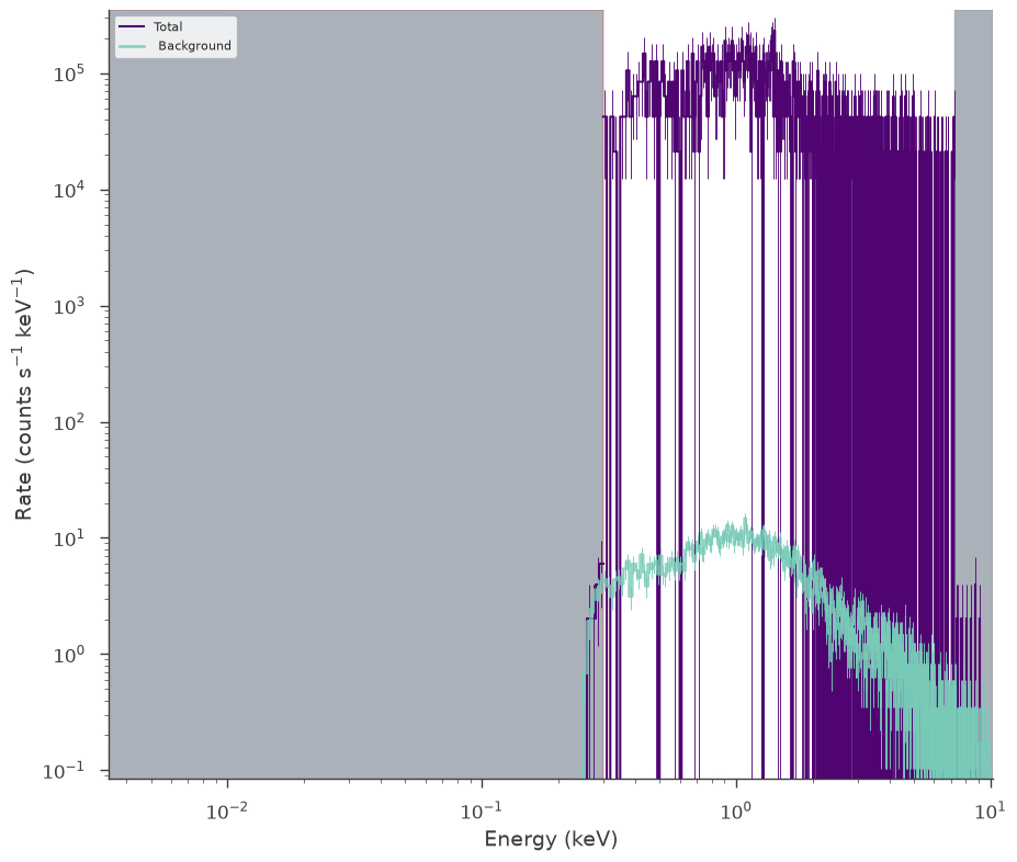
fit = xrt.view_count_spectrum(scale_background=False)

../_images/notebooks_joint_fitting_xrt_and_gbm_xspec_models_6_0.png

Load GBM data

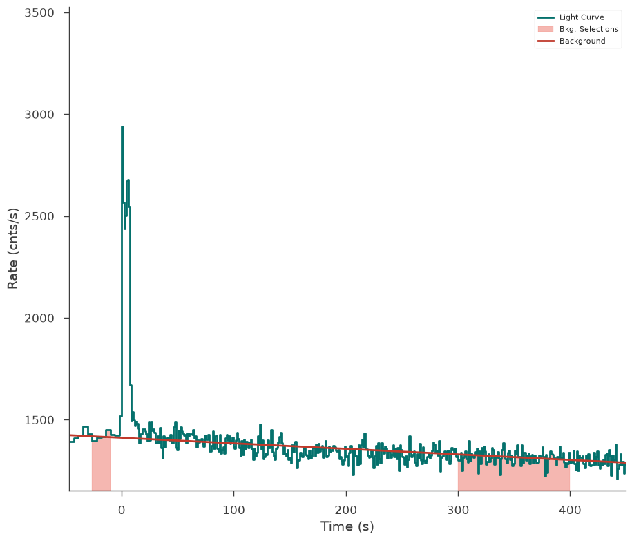
Load all the GBM data you need and make appropriate background, source time, and energy selections. Make sure to check the light curves!

[6]:

trigger_number = "bn110731465"
gbm_data = download_GBM_trigger_data(trigger_number, detectors=["n3"])

[7]:

# Select the time interval
src_selection = "100.169342-150.169342"
bkg_selection = ["-25.0--10.0", "300-400"]
ts = TimeSeriesBuilder.from_gbm_cspec_or_ctime(
    name="gbm_n3",
    cspec_or_ctime_file=gbm_data["n3"]["cspec"],
    rsp_file=gbm_data["n3"]["rsp"],
)


ts.set_background_interval(*bkg_selection)
ts.save_background("n3_bkg.h5", overwrite=True)
fig = ts.view_lightcurve(-50, 450)

The default choice for MATRIX extension failed:KeyError("Extension ('MATRIX', 1) not found.")available: None 'EBOUNDS' 'SPECRESP MATRIX' 'SPECRESP MATRIX' 'SPECRESP MATRIX' 'SPECRESP MATRIX' 'SPECRESP MATRIX' 'SPECRESP MATRIX' 'SPECRESP MATRIX' 'SPECRESP MATRIX' 'SPECRESP MATRIX' 'SPECRESP MATRIX' 'SPECRESP MATRIX'
No TLMIN keyword found. This DRM does not follow OGIP standards. Assuming TLMIN=1
Minimum MC energy (5.0) is larger than minimum EBOUNDS energy (4.2829999923706055)

The default choice for MATRIX extension failed:KeyError("Extension ('MATRIX', 1) not found.")available: None 'EBOUNDS' 'SPECRESP MATRIX' 'SPECRESP MATRIX' 'SPECRESP MATRIX' 'SPECRESP MATRIX' 'SPECRESP MATRIX' 'SPECRESP MATRIX' 'SPECRESP MATRIX' 'SPECRESP MATRIX' 'SPECRESP MATRIX' 'SPECRESP MATRIX' 'SPECRESP MATRIX'
No TLMIN keyword found. This DRM does not follow OGIP standards. Assuming TLMIN=1
Minimum MC energy (5.0) is larger than minimum EBOUNDS energy (4.2829999923706055)
The default choice for MATRIX extension failed:KeyError("Extension ('MATRIX', 2) not found.")available: None 'EBOUNDS' 'SPECRESP MATRIX' 'SPECRESP MATRIX' 'SPECRESP MATRIX' 'SPECRESP MATRIX' 'SPECRESP MATRIX' 'SPECRESP MATRIX' 'SPECRESP MATRIX' 'SPECRESP MATRIX' 'SPECRESP MATRIX' 'SPECRESP MATRIX' 'SPECRESP MATRIX'
No TLMIN keyword found. This DRM does not follow OGIP standards. Assuming TLMIN=1
Minimum MC energy (5.0) is larger than minimum EBOUNDS energy (4.2829999923706055)
The default choice for MATRIX extension failed:KeyError("Extension ('MATRIX', 3) not found.")available: None 'EBOUNDS' 'SPECRESP MATRIX' 'SPECRESP MATRIX' 'SPECRESP MATRIX' 'SPECRESP MATRIX' 'SPECRESP MATRIX' 'SPECRESP MATRIX' 'SPECRESP MATRIX' 'SPECRESP MATRIX' 'SPECRESP MATRIX' 'SPECRESP MATRIX' 'SPECRESP MATRIX'
No TLMIN keyword found. This DRM does not follow OGIP standards. Assuming TLMIN=1
Minimum MC energy (5.0) is larger than minimum EBOUNDS energy (4.2829999923706055)
The default choice for MATRIX extension failed:KeyError("Extension ('MATRIX', 4) not found.")available: None 'EBOUNDS' 'SPECRESP MATRIX' 'SPECRESP MATRIX' 'SPECRESP MATRIX' 'SPECRESP MATRIX' 'SPECRESP MATRIX' 'SPECRESP MATRIX' 'SPECRESP MATRIX' 'SPECRESP MATRIX' 'SPECRESP MATRIX' 'SPECRESP MATRIX' 'SPECRESP MATRIX'
No TLMIN keyword found. This DRM does not follow OGIP standards. Assuming TLMIN=1
Minimum MC energy (5.0) is larger than minimum EBOUNDS energy (4.2829999923706055)
The default choice for MATRIX extension failed:KeyError("Extension ('MATRIX', 5) not found.")available: None 'EBOUNDS' 'SPECRESP MATRIX' 'SPECRESP MATRIX' 'SPECRESP MATRIX' 'SPECRESP MATRIX' 'SPECRESP MATRIX' 'SPECRESP MATRIX' 'SPECRESP MATRIX' 'SPECRESP MATRIX' 'SPECRESP MATRIX' 'SPECRESP MATRIX' 'SPECRESP MATRIX'
No TLMIN keyword found. This DRM does not follow OGIP standards. Assuming TLMIN=1
Minimum MC energy (5.0) is larger than minimum EBOUNDS energy (4.2829999923706055)
The default choice for MATRIX extension failed:KeyError("Extension ('MATRIX', 6) not found.")available: None 'EBOUNDS' 'SPECRESP MATRIX' 'SPECRESP MATRIX' 'SPECRESP MATRIX' 'SPECRESP MATRIX' 'SPECRESP MATRIX' 'SPECRESP MATRIX' 'SPECRESP MATRIX' 'SPECRESP MATRIX' 'SPECRESP MATRIX' 'SPECRESP MATRIX' 'SPECRESP MATRIX'
No TLMIN keyword found. This DRM does not follow OGIP standards. Assuming TLMIN=1
Minimum MC energy (5.0) is larger than minimum EBOUNDS energy (4.2829999923706055)
The default choice for MATRIX extension failed:KeyError("Extension ('MATRIX', 7) not found.")available: None 'EBOUNDS' 'SPECRESP MATRIX' 'SPECRESP MATRIX' 'SPECRESP MATRIX' 'SPECRESP MATRIX' 'SPECRESP MATRIX' 'SPECRESP MATRIX' 'SPECRESP MATRIX' 'SPECRESP MATRIX' 'SPECRESP MATRIX' 'SPECRESP MATRIX' 'SPECRESP MATRIX'
No TLMIN keyword found. This DRM does not follow OGIP standards. Assuming TLMIN=1
Minimum MC energy (5.0) is larger than minimum EBOUNDS energy (4.2829999923706055)
The default choice for MATRIX extension failed:KeyError("Extension ('MATRIX', 8) not found.")available: None 'EBOUNDS' 'SPECRESP MATRIX' 'SPECRESP MATRIX' 'SPECRESP MATRIX' 'SPECRESP MATRIX' 'SPECRESP MATRIX' 'SPECRESP MATRIX' 'SPECRESP MATRIX' 'SPECRESP MATRIX' 'SPECRESP MATRIX' 'SPECRESP MATRIX' 'SPECRESP MATRIX'
No TLMIN keyword found. This DRM does not follow OGIP standards. Assuming TLMIN=1
Minimum MC energy (5.0) is larger than minimum EBOUNDS energy (4.2829999923706055)
The default choice for MATRIX extension failed:KeyError("Extension ('MATRIX', 9) not found.")available: None 'EBOUNDS' 'SPECRESP MATRIX' 'SPECRESP MATRIX' 'SPECRESP MATRIX' 'SPECRESP MATRIX' 'SPECRESP MATRIX' 'SPECRESP MATRIX' 'SPECRESP MATRIX' 'SPECRESP MATRIX' 'SPECRESP MATRIX' 'SPECRESP MATRIX' 'SPECRESP MATRIX'
No TLMIN keyword found. This DRM does not follow OGIP standards. Assuming TLMIN=1
Minimum MC energy (5.0) is larger than minimum EBOUNDS energy (4.2829999923706055)
The default choice for MATRIX extension failed:KeyError("Extension ('MATRIX', 10) not found.")available: None 'EBOUNDS' 'SPECRESP MATRIX' 'SPECRESP MATRIX' 'SPECRESP MATRIX' 'SPECRESP MATRIX' 'SPECRESP MATRIX' 'SPECRESP MATRIX' 'SPECRESP MATRIX' 'SPECRESP MATRIX' 'SPECRESP MATRIX' 'SPECRESP MATRIX' 'SPECRESP MATRIX'
No TLMIN keyword found. This DRM does not follow OGIP standards. Assuming TLMIN=1
Minimum MC energy (5.0) is larger than minimum EBOUNDS energy (4.2829999923706055)
The default choice for MATRIX extension failed:KeyError("Extension ('MATRIX', 11) not found.")available: None 'EBOUNDS' 'SPECRESP MATRIX' 'SPECRESP MATRIX' 'SPECRESP MATRIX' 'SPECRESP MATRIX' 'SPECRESP MATRIX' 'SPECRESP MATRIX' 'SPECRESP MATRIX' 'SPECRESP MATRIX' 'SPECRESP MATRIX' 'SPECRESP MATRIX' 'SPECRESP MATRIX'
No TLMIN keyword found. This DRM does not follow OGIP standards. Assuming TLMIN=1
Minimum MC energy (5.0) is larger than minimum EBOUNDS energy (4.2829999923706055)
Minimum MC energy (5.0) is larger than minimum EBOUNDS energy (4.2829999923706055)

../_images/notebooks_joint_fitting_xrt_and_gbm_xspec_models_9_5.png

[8]:

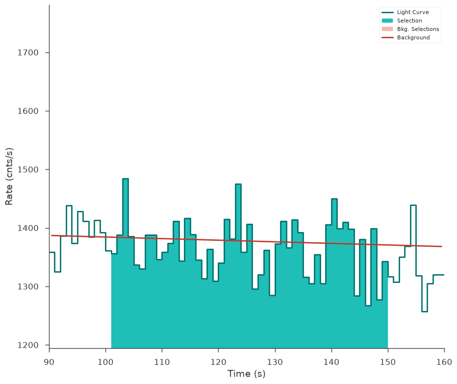
ts = TimeSeriesBuilder.from_gbm_tte(
    "gbm_n3",
    tte_file=gbm_data["n3"]["tte"],
    rsp_file=gbm_data["n3"]["rsp"],
    restore_background="n3_bkg.h5",
)


ts.set_active_time_interval(src_selection)

fig = ts.view_lightcurve(90, 160)

The TTE file /home/runner/work/threeML/threeML/docs/md_docs/slow_execute/glg_tte_n3_bn110731465_v00.fit.gz contains duplicate time tags and is thus invalid. Contact the FSSC
The default choice for MATRIX extension failed:KeyError("Extension ('MATRIX', 1) not found.")available: None 'EBOUNDS' 'SPECRESP MATRIX' 'SPECRESP MATRIX' 'SPECRESP MATRIX' 'SPECRESP MATRIX' 'SPECRESP MATRIX' 'SPECRESP MATRIX' 'SPECRESP MATRIX' 'SPECRESP MATRIX' 'SPECRESP MATRIX' 'SPECRESP MATRIX' 'SPECRESP MATRIX'
No TLMIN keyword found. This DRM does not follow OGIP standards. Assuming TLMIN=1
Minimum MC energy (5.0) is larger than minimum EBOUNDS energy (4.2829999923706055)
The default choice for MATRIX extension failed:KeyError("Extension ('MATRIX', 2) not found.")available: None 'EBOUNDS' 'SPECRESP MATRIX' 'SPECRESP MATRIX' 'SPECRESP MATRIX' 'SPECRESP MATRIX' 'SPECRESP MATRIX' 'SPECRESP MATRIX' 'SPECRESP MATRIX' 'SPECRESP MATRIX' 'SPECRESP MATRIX' 'SPECRESP MATRIX' 'SPECRESP MATRIX'
No TLMIN keyword found. This DRM does not follow OGIP standards. Assuming TLMIN=1
Minimum MC energy (5.0) is larger than minimum EBOUNDS energy (4.2829999923706055)
The default choice for MATRIX extension failed:KeyError("Extension ('MATRIX', 3) not found.")available: None 'EBOUNDS' 'SPECRESP MATRIX' 'SPECRESP MATRIX' 'SPECRESP MATRIX' 'SPECRESP MATRIX' 'SPECRESP MATRIX' 'SPECRESP MATRIX' 'SPECRESP MATRIX' 'SPECRESP MATRIX' 'SPECRESP MATRIX' 'SPECRESP MATRIX' 'SPECRESP MATRIX'
No TLMIN keyword found. This DRM does not follow OGIP standards. Assuming TLMIN=1
Minimum MC energy (5.0) is larger than minimum EBOUNDS energy (4.2829999923706055)
The default choice for MATRIX extension failed:KeyError("Extension ('MATRIX', 4) not found.")available: None 'EBOUNDS' 'SPECRESP MATRIX' 'SPECRESP MATRIX' 'SPECRESP MATRIX' 'SPECRESP MATRIX' 'SPECRESP MATRIX' 'SPECRESP MATRIX' 'SPECRESP MATRIX' 'SPECRESP MATRIX' 'SPECRESP MATRIX' 'SPECRESP MATRIX' 'SPECRESP MATRIX'
No TLMIN keyword found. This DRM does not follow OGIP standards. Assuming TLMIN=1
Minimum MC energy (5.0) is larger than minimum EBOUNDS energy (4.2829999923706055)
The default choice for MATRIX extension failed:KeyError("Extension ('MATRIX', 5) not found.")available: None 'EBOUNDS' 'SPECRESP MATRIX' 'SPECRESP MATRIX' 'SPECRESP MATRIX' 'SPECRESP MATRIX' 'SPECRESP MATRIX' 'SPECRESP MATRIX' 'SPECRESP MATRIX' 'SPECRESP MATRIX' 'SPECRESP MATRIX' 'SPECRESP MATRIX' 'SPECRESP MATRIX'
No TLMIN keyword found. This DRM does not follow OGIP standards. Assuming TLMIN=1
Minimum MC energy (5.0) is larger than minimum EBOUNDS energy (4.2829999923706055)
The default choice for MATRIX extension failed:KeyError("Extension ('MATRIX', 6) not found.")available: None 'EBOUNDS' 'SPECRESP MATRIX' 'SPECRESP MATRIX' 'SPECRESP MATRIX' 'SPECRESP MATRIX' 'SPECRESP MATRIX' 'SPECRESP MATRIX' 'SPECRESP MATRIX' 'SPECRESP MATRIX' 'SPECRESP MATRIX' 'SPECRESP MATRIX' 'SPECRESP MATRIX'
No TLMIN keyword found. This DRM does not follow OGIP standards. Assuming TLMIN=1
Minimum MC energy (5.0) is larger than minimum EBOUNDS energy (4.2829999923706055)
The default choice for MATRIX extension failed:KeyError("Extension ('MATRIX', 7) not found.")available: None 'EBOUNDS' 'SPECRESP MATRIX' 'SPECRESP MATRIX' 'SPECRESP MATRIX' 'SPECRESP MATRIX' 'SPECRESP MATRIX' 'SPECRESP MATRIX' 'SPECRESP MATRIX' 'SPECRESP MATRIX' 'SPECRESP MATRIX' 'SPECRESP MATRIX' 'SPECRESP MATRIX'
No TLMIN keyword found. This DRM does not follow OGIP standards. Assuming TLMIN=1
Minimum MC energy (5.0) is larger than minimum EBOUNDS energy (4.2829999923706055)
The default choice for MATRIX extension failed:KeyError("Extension ('MATRIX', 8) not found.")available: None 'EBOUNDS' 'SPECRESP MATRIX' 'SPECRESP MATRIX' 'SPECRESP MATRIX' 'SPECRESP MATRIX' 'SPECRESP MATRIX' 'SPECRESP MATRIX' 'SPECRESP MATRIX' 'SPECRESP MATRIX' 'SPECRESP MATRIX' 'SPECRESP MATRIX' 'SPECRESP MATRIX'
No TLMIN keyword found. This DRM does not follow OGIP standards. Assuming TLMIN=1
Minimum MC energy (5.0) is larger than minimum EBOUNDS energy (4.2829999923706055)
The default choice for MATRIX extension failed:KeyError("Extension ('MATRIX', 9) not found.")available: None 'EBOUNDS' 'SPECRESP MATRIX' 'SPECRESP MATRIX' 'SPECRESP MATRIX' 'SPECRESP MATRIX' 'SPECRESP MATRIX' 'SPECRESP MATRIX' 'SPECRESP MATRIX' 'SPECRESP MATRIX' 'SPECRESP MATRIX' 'SPECRESP MATRIX' 'SPECRESP MATRIX'
No TLMIN keyword found. This DRM does not follow OGIP standards. Assuming TLMIN=1
Minimum MC energy (5.0) is larger than minimum EBOUNDS energy (4.2829999923706055)
The default choice for MATRIX extension failed:KeyError("Extension ('MATRIX', 10) not found.")available: None 'EBOUNDS' 'SPECRESP MATRIX' 'SPECRESP MATRIX' 'SPECRESP MATRIX' 'SPECRESP MATRIX' 'SPECRESP MATRIX' 'SPECRESP MATRIX' 'SPECRESP MATRIX' 'SPECRESP MATRIX' 'SPECRESP MATRIX' 'SPECRESP MATRIX' 'SPECRESP MATRIX'
No TLMIN keyword found. This DRM does not follow OGIP standards. Assuming TLMIN=1
Minimum MC energy (5.0) is larger than minimum EBOUNDS energy (4.2829999923706055)
The default choice for MATRIX extension failed:KeyError("Extension ('MATRIX', 11) not found.")available: None 'EBOUNDS' 'SPECRESP MATRIX' 'SPECRESP MATRIX' 'SPECRESP MATRIX' 'SPECRESP MATRIX' 'SPECRESP MATRIX' 'SPECRESP MATRIX' 'SPECRESP MATRIX' 'SPECRESP MATRIX' 'SPECRESP MATRIX' 'SPECRESP MATRIX' 'SPECRESP MATRIX'
No TLMIN keyword found. This DRM does not follow OGIP standards. Assuming TLMIN=1
Minimum MC energy (5.0) is larger than minimum EBOUNDS energy (4.2829999923706055)
Minimum MC energy (5.0) is larger than minimum EBOUNDS energy (4.2829999923706055)
Minimum MC energy (5.0) is larger than minimum EBOUNDS energy (4.2829999923706055)

../_images/notebooks_joint_fitting_xrt_and_gbm_xspec_models_10_1.png

[9]:

nai3 = ts.to_spectrumlike()

Make energy selections and check them out

[10]:

nai3.set_active_measurements("8-900")
fig = nai3.view_count_spectrum()

../_images/notebooks_joint_fitting_xrt_and_gbm_xspec_models_13_0.png

Setup the model

astromodels allows you to use XSPEC models if you have XSPEC installed. Set all the normal parameters you would in XSPEC and build a model the normal 3ML/astromodels way! Here we will use the phabs model from XSPEC and mix it with powerlaw model in astromodels.

With XSPEC

[11]:

xspec_abund("angr")

spectral_model = XS_phabs() * XS_zphabs() * Powerlaw()
spectral_model.set_units(u.keV, 1 / (u.keV * u.cm**2 * u.s))

spectral_model.nh_1 = 0.101
spectral_model.nh_1.bounds = (None, None)
spectral_model.nh_1.fix = True

spectral_model.nh_2 = 0.1114424
spectral_model.nh_2.fix = True
spectral_model.nh_2.bounds = (None, None)
spectral_model.redshift_2 = 0.618
spectral_model.redshift_2.fix = True

 Solar Abundance Vector set to angr:  Anders E. & Grevesse N. Geochimica et Cosmochimica Acta 53, 197 (1989)

With astromodels PHABS

We can build the exact same models in native astromodels thanks to Dominique Eckert. Here, there is no extra function for redshifting the absorption model, just pass a redshift.

[12]:

phabs_local = PhAbs(NH=0.101)
phabs_local.NH.fix = True
phabs_local.redshift.fix = True
phabs_src = PhAbs(NH=0.1114424, redshift=0.618)
phabs_src.NH.fix = True
phabs_src.redshift.fix = True
pl = Powerlaw()
spectral_model_native = phabs_local * phabs_src * pl

Setup the joint likelihood

Create a point source object and model.

Load the data into a data list and create the joint likelihood

With XSPEC models

First we will fit with the XSPEC model

[13]:

ptsrc = PointSource(trigger, ra, dec, spectral_shape=spectral_model)
model = Model(ptsrc)

[14]:

data = DataList(xrt, nai3)

jl = JointLikelihood(model, data, verbose=False)
model.display()

Model summary:

	N
Point sources	1
Extended sources	0
Particle sources	0

Free parameters (2):

	value	min_value	max_value	unit
GRB110731A.spectrum.main.composite.K_3	1.0	0.0	1000.0	keV-1 s-1 cm-2
GRB110731A.spectrum.main.composite.index_3	-2.01	-10.0	10.0

Fixed parameters (8):
(abridged. Use complete=True to see all fixed parameters)

Properties (0):

(none)

Linked parameters (0):

(none)

Independent variables:

(none)

Linked functions (0):

(none)

[15]:

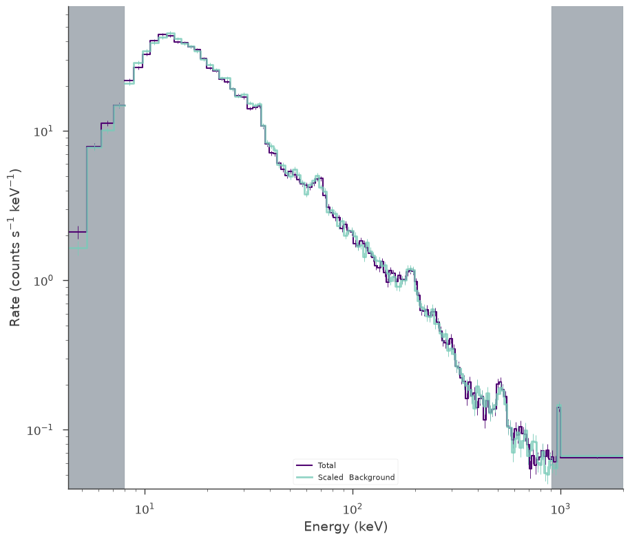
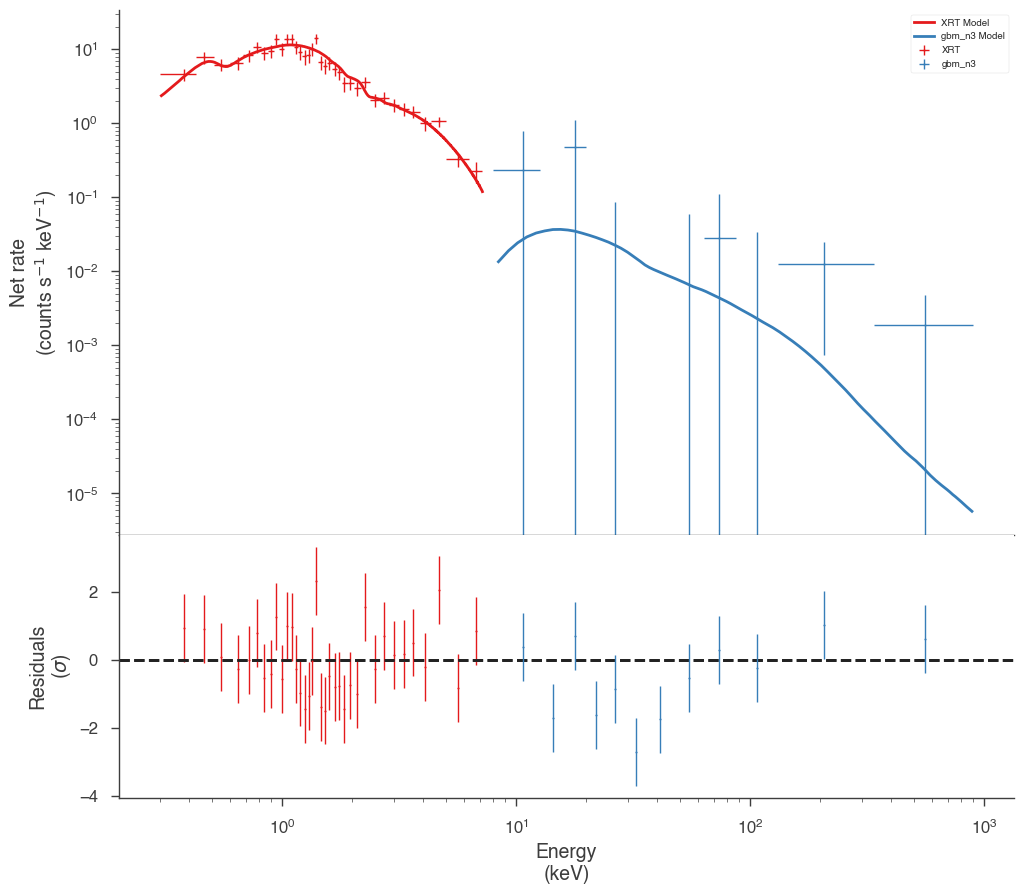
res = jl.fit()
fig = display_spectrum_model_counts(jl, min_rate=[0.5, 0.1])

Best fit values:

	result	unit
parameter
GRB110731A.spectrum.main.composite.K_3	(1.83 +/- 0.07) x 10^-1	1 / (keV s cm2)
GRB110731A.spectrum.main.composite.index_3	-1.93 +/- 0.05

Correlation matrix:

1.00	-0.57
-0.57	1.00

Values of -log(likelihood) at the minimum:

	-log(likelihood)
XRT	2064.191129
gbm_n3	983.140112
total	3047.331241

Values of statistical measures:

	statistical measures
AIC	6098.677371
BIC	6108.054080

../_images/notebooks_joint_fitting_xrt_and_gbm_xspec_models_24_8.png

[16]:

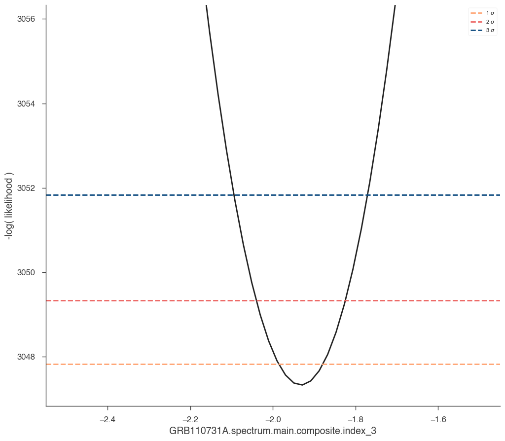
res = jl.get_contours(spectral_model.index_3, -2.5, -1.5, 50)

../_images/notebooks_joint_fitting_xrt_and_gbm_xspec_models_25_1.png

[17]:

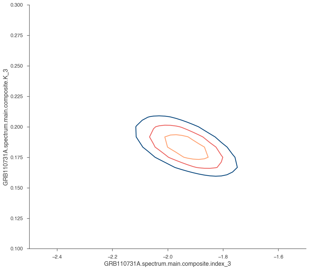
_ = jl.get_contours(
    spectral_model.K_3, 0.1, 0.3, 25, spectral_model.index_3, -2.5, -1.5, 50
)

../_images/notebooks_joint_fitting_xrt_and_gbm_xspec_models_26_1.png

[18]:

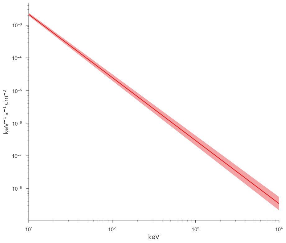
fig = plot_spectra(jl.results, show_legend=False, emin=0.01 * u.keV)

../_images/notebooks_joint_fitting_xrt_and_gbm_xspec_models_27_2.png

Fit with astromodels PhAbs

Now lets repeat the fit in pure astromodels.

[19]:

ptsrc_native = PointSource(trigger, ra, dec, spectral_shape=spectral_model_native)
model_native = Model(ptsrc_native)

[20]:

data = DataList(xrt, nai3)

jl_native = JointLikelihood(model_native, data, verbose=False)
model.display()

Model summary:

	N
Point sources	1
Extended sources	0
Particle sources	0

Free parameters (2):

	value	min_value	max_value	unit
GRB110731A.spectrum.main.composite.K_3	0.183083	0.0	1000.0	keV-1 s-1 cm-2
GRB110731A.spectrum.main.composite.index_3	-1.932241	-10.0	10.0

Fixed parameters (8):
(abridged. Use complete=True to see all fixed parameters)

Properties (0):

(none)

Linked parameters (0):

(none)

Independent variables:

(none)

Linked functions (0):

(none)

[21]:

res = jl_native.fit()
fig = display_spectrum_model_counts(jl_native, min_rate=[0.5, 0.1])

Best fit values:

	result	unit
parameter
GRB110731A.spectrum.main.composite.K_3	(1.83 +/- 0.07) x 10^-1	1 / (keV s cm2)
GRB110731A.spectrum.main.composite.index_3	-1.93 +/- 0.05

Correlation matrix:

1.00	-0.57
-0.57	1.00

Values of -log(likelihood) at the minimum:

	-log(likelihood)
XRT	2064.181385
gbm_n3	983.140032
total	3047.321417

Values of statistical measures:

	statistical measures
AIC	6098.657722
BIC	6108.034432

../_images/notebooks_joint_fitting_xrt_and_gbm_xspec_models_32_8.png

[22]:

fig = plot_spectra(jl.results, jl_native.results, show_legend=False, emin=0.01 * u.keV)

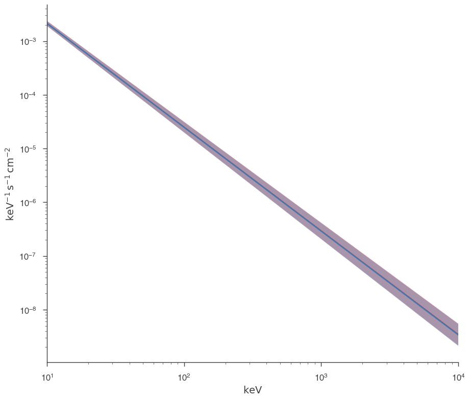
../_images/notebooks_joint_fitting_xrt_and_gbm_xspec_models_33_3.png

Both approaches give the same answer as they should.

[ ]: